3D Reconstruction of the Human Rib Cage from 2D Projection ... - ZIB

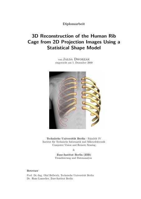
Diplomarbeit
3D Reconstruction of the Human Rib
Cage from 2D Projection Images Using a
Statistical Shape Model
Betreuer
von Jalda Dworzak
eingereicht am 5. Dezember 2009
Technische Universität Berlin - Fakultät IV
Institut für Technische Informatik und Mikroelektronik
Computer Vision and Remote Sensing
&
Zuse-Institut Berlin (ZIB)
Visualisierung und Datenanalyse
Prof. Dr.-Ing. Olaf Hellwich, Technische Universität Berlin
Dr. Hans Lamecker, Zuse-Institut Berlin

Die selbständige und eigenhändige Anfertigung versichere ich an Eides Statt.
Berlin, 5. Dezember 2009
iii

Abstract
This diploma thesis presents an approach for the three-dimensional (3D) shape and
pose reconstruction of the human rib cage from few segmented two-dimensional
(2D) projection images. The work is aimed at supporting temporal subtraction
techniques of subsequently acquired radiographs by establishing a method for the
assessment of pose differences in sequences of chest radiographs of the same patient.
The reconstruction method is based on a 3D statistical shape model (SSM)
of the rib cage, which is adapted to 2D projection images of an individual rib cage.
To drive the adaptation, a distance measure is minimized that quantifies the dissimilarities
between 2D projections of the 3D SSM and the 2D projection images.
Different silhouette-based distance measures are proposed and evaluated regarding
their suitability for the adaptation of the SSM to the projection images. An evaluation
was performed on 29 sets of biplanar binary images (posterior-anterior and
lateral) as well as on posterior-anterior X-ray images of a phantom of a human rib
cage. Depending on the chosen distance measure, our experiments on the combined
reconstruction of shape and pose of the rib cages yield reconstruction accuracies
from 2.2 mm to 4.7 mm average mean 3D surface distance. Given a geometry of an
individual rib cage, the rotational errors for the pose reconstruction range from 0.1 ◦
to 0.9 ◦ . In conclusion, the results show that the proposed method is suitable for the
estimation of pose differences of the human rib cage in projection images. Thus, it
is able to provide crucial 3D information for the registration during the generation
of 2D subtraction images.
iv

Deutsche Zusammenfassung
Im Rahmen dieser Diplomarbeit wurde ein Verfahren zur dreidimensionalen (3D)
Rekonstruktion der Lage und Form des menschlichen Brustkorbes aus wenigen zweidimensionalen
(2D) Projektionsbildern entwickelt und implementiert. Ziel der Arbeit
ist es, durch die Bereitstellung einer Methode zur Ermittlung von 3D-
Lageunterschieden zwischen zeitlich versetzt aufgenommenen Thoraxradiographien,
diagnostische Bildsubtraktionsverfahren zu unterstützen und zu verbessern. Die
Rekonstruktionsmethode basiert auf einem statistischen 3D-Formmodell (SFM) der
Rippen, das zum Zwecke der Rekonstruktion in eine Bildebene projeziert und an die
2D-Bilddaten eines individuellen Brustkorbes angepasst wird. Diese Anpassung wird
durch die Minimierung eines Distanzmaßes gesteuert, das Unterschiede zwischen
Projektionen des SFMs und den 2D-Projektionsdaten misst. Hierfür wurden unterschiedliche
Silhouetten-basierte Distanzmaße entwickelt und hinsichtlich ihrer Anwendbarkeit
auf das Rekonstruktionsproblem ausgewertet. Eine Validierung des Verfahrens
wurde mit Hilfe von 29 künstlich generierten Paaren biplanarer Binärbilder
(Frontal- und Seitenansicht) sowie mit Radiographien (nur Frontalansicht) eines
Thoraxmodells (Phantom) durchgeführt. Experimente zur gleichzeitigen Ermittlung
von Form und Lage eines Brustkorbes erreichen, in Abhängigkeit des gewählten
Distanzmaßes, eine Rekonstruktionsgenauigkeit zwischen 2.2 bis 4.7 mm mittlerer
3D-Oberflächendistanz. Ist die Form bereits vor der Anpassung bekannt, ergibt eine
reine Lageabschätzung Rotationsfehler im Bereich von 0.1 ◦ bis 0.9 ◦ . Die Ergebnisse
zeigen, dass die vorgeschlagene Methode für die Abschätzung von Lageunterschieden
in Röntgenbildern des menschlichen Thorax geeignet ist. Folglich können mit Hilfe
des Rekonstruktionsverfahrens entscheidende 3D-Information für die Generierung
von 2D-Subtraktionsbildern, mit Anwendung in der computergestützten, medizinischen
Diagnose, gewonnen werden.
v

Acknowledgements
On a first note of my diploma thesis, I want to express my gratitude to my supervisor
Dr. Hans Lamecker whose work was the starting point and basis of this thesis and
who provided me with indispensable support and feedback. My sincere thanks go
to Prof. Dr.-Ing. Olaf Hellwich for his valuable advice and for allowing me to pursue
my graduate work under his supervision.
I am indebted to Hans-Christian Hege who enabled me to work in the extremely
resourceful environment of the Visualization an Data Analysis Group at the Zuse-
Institute Berlin (ZIB). The pleasant and inspiring atmosphere created by all the
members of my department is greatly appreciated. Furthermore, I want to thank
Dr. Stefan Zachow who provided me with excellent guidance and in whose Medical
Planning Group I learned a great deal about computer-aided surgery and diagnosis
as well as medical image analysis.
I am especially grateful for the exceptional help and constant encouragement I
received from my collegues Dagmar Kainmüller and Heiko Seim. Thank you for
sharing your time on countless occasions and for being so patient with me!
The work of this thesis would not have been possible without the cooperation
between the Department of Medical Imaging Systems at Philips Research Europe
in Hamburg and the Visualization and Data Analysis Group at ZIB in Berlin. I
am very much obliged to Dr. Jens von Berg, Dr. Cristian Lorenz, Tobias Klinder
and Dennis Barthel for giving me the opportunity to work on such an exiting and
application-oriented topic, for sharing their great expertise and making my stays in
Hamburg fruitful and enjoyable. Further thanks go to Dr. Cornelia Schaefer-Prokop
for providing the radiographs.
Last but definitely not least, I wish to thank my family and friends for their
support.
vi

Contents
1 Introduction 1
1.1 Motivation . . . . . . . . . . . . . . . . . . . . . . . . . . . . . . . . 1
1.2 Problem and Objectives . . . . . . . . . . . . . . . . . . . . . . . . . 2
1.3 Contribution . . . . . . . . . . . . . . . . . . . . . . . . . . . . . . . 4
1.4 Overview . . . . . . . . . . . . . . . . . . . . . . . . . . . . . . . . . 6
2 Medical Background 7
2.1 Anatomy and Functionality of the Rib Cage . . . . . . . . . . . . . . 7
2.2 Chest Radiography . . . . . . . . . . . . . . . . . . . . . . . . . . . . 8
2.3 Image Subtraction in CAD . . . . . . . . . . . . . . . . . . . . . . . 10
2.4 Requirements and Challenges . . . . . . . . . . . . . . . . . . . . . . 11
3 Related Work 13
3.1 Reconstruction of the Rib Cage from X-ray Images . . . . . . . . . . 13
3.2 2D/3D Reconstruction . . . . . . . . . . . . . . . . . . . . . . . . . . 15
3.2.1 Pose Reconstruction . . . . . . . . . . . . . . . . . . . . . . . 16
3.2.2 Shape Reconstruction . . . . . . . . . . . . . . . . . . . . . . 17
3.3 Distance Measures . . . . . . . . . . . . . . . . . . . . . . . . . . . . 18
3.3.1 Intensity-based Methods . . . . . . . . . . . . . . . . . . . . . 18
3.3.2 Feature-based Methods . . . . . . . . . . . . . . . . . . . . . 19
3.3.3 Building Correspondences . . . . . . . . . . . . . . . . . . . . 19
4 SSM-based Geometry Reconstruction from 2D Projection Images 23
4.1 Reconstruction Process . . . . . . . . . . . . . . . . . . . . . . . . . . 23
4.2 Preliminaries . . . . . . . . . . . . . . . . . . . . . . . . . . . . . . . 25
4.2.1 Transformation Parameterization . . . . . . . . . . . . . . . . 25
4.3 Statistical Shape Models . . . . . . . . . . . . . . . . . . . . . . . . . 27
4.3.1 Statistical Shape Modeling . . . . . . . . . . . . . . . . . . . 27
4.3.2 Quality Requirements for SSMs . . . . . . . . . . . . . . . . . 30
4.3.3 Fields of Applications . . . . . . . . . . . . . . . . . . . . . . 30
4.4 Projection of SSMs . . . . . . . . . . . . . . . . . . . . . . . . . . . . 30
4.5 Optimization . . . . . . . . . . . . . . . . . . . . . . . . . . . . . . . 32
4.5.1 Gradient Descent . . . . . . . . . . . . . . . . . . . . . . . . . 33
4.5.2 Multilevel Approaches . . . . . . . . . . . . . . . . . . . . . . 34
5 Reconstruction of the Human Rib Cage from X-ray Images 35
5.1 Statistical Shape Model of the Rib Cage . . . . . . . . . . . . . . . . 35
5.2 Distance Measures . . . . . . . . . . . . . . . . . . . . . . . . . . . . 35
5.2.1 Silhouettes . . . . . . . . . . . . . . . . . . . . . . . . . . . . 36
5.2.2 Symmetric and Asymmetric Distance Measures . . . . . . . . 37
vii

5.2.3 Contour Normals . . . . . . . . . . . . . . . . . . . . . . . . . 37
5.2.4 Difference in Area . . . . . . . . . . . . . . . . . . . . . . . . 37
5.3 Distance Computation . . . . . . . . . . . . . . . . . . . . . . . . . . 38
5.4 Initialization . . . . . . . . . . . . . . . . . . . . . . . . . . . . . . . 39
6 Experiments and Results 43
6.1 Evaluation of Distance Measures . . . . . . . . . . . . . . . . . . . . 43
6.1.1 Sampling of the Parameter Space . . . . . . . . . . . . . . . . 43
6.1.2 Choice of Distance Measure . . . . . . . . . . . . . . . . . . . 46
6.2 Reconstruction Accuracy and Robustness . . . . . . . . . . . . . . . 47
6.2.1 Experimental Setup . . . . . . . . . . . . . . . . . . . . . . . 48
6.2.2 Evaluation Measures . . . . . . . . . . . . . . . . . . . . . . . 48
6.2.3 Initialization . . . . . . . . . . . . . . . . . . . . . . . . . . . 50
6.2.4 3D Pose Reconstruction . . . . . . . . . . . . . . . . . . . . . 51
6.2.5 3D Shape and Pose Reconstruction . . . . . . . . . . . . . . . 53
6.3 Reconstruction from Radiographs . . . . . . . . . . . . . . . . . . . . 56
6.3.1 X-ray Images of a Thorax Phantom . . . . . . . . . . . . . . 56
6.3.2 3D Pose Reconstruction . . . . . . . . . . . . . . . . . . . . . 56
6.3.3 Exemplary Reconstruction from Clinical X-ray Images . . . . 58
7 Discussion and Future Work 61
7.1 Methodological Findings . . . . . . . . . . . . . . . . . . . . . . . . . 61
7.1.1 Accuracy of Pose Reconstruction . . . . . . . . . . . . . . . . 61
7.1.2 Accuracy of Shape Reconstruction . . . . . . . . . . . . . . . 61
7.1.3 Comparison with Other Methods . . . . . . . . . . . . . . . . 63
7.2 Application to the Clinics . . . . . . . . . . . . . . . . . . . . . . . . 63
8 Conclusions 67
Bibliography 69
viii

List of Figures
1.1 Subtraction images to detect interval changes . . . . . . . . . . . . . 2
1.2 Assessing 3D pose differences . . . . . . . . . . . . . . . . . . . . . . 3
1.3 The general idea of the reconstruction scheme . . . . . . . . . . . . . 5
2.1 Components of the rib cage . . . . . . . . . . . . . . . . . . . . . . . 7
2.2 Standard posterior-anterior and lateral X-ray images . . . . . . . . . 8
2.3 The cortical bone layer . . . . . . . . . . . . . . . . . . . . . . . . . . 9
2.4 Spot the difference – toy example for a subtraction image . . . . . . 10
2.5 Impact of differences in the patient’s 3D pose to 2D image registration 11
2.6 Temporal subtraction CAD system . . . . . . . . . . . . . . . . . . . 12
3.1 Image acquisition geometry for stereo-radiographs, Delorme et al. . . 14
3.2 Reconstruction of the rib midlines, Benameur et al. . . . . . . . . . . 14
3.3 3D template fitting according to Koehler et al. . . . . . . . . . . . . 15
3.4 Shape reconstruction of the pelvis according to Lamecker et al. . . . 17
3.5 3D to 3D correspondence building according to Zhang et al. . . . . . 21
3.6 Point correspondences . . . . . . . . . . . . . . . . . . . . . . . . . . 21
4.1 Scheme of the SSM-based reconstruction process . . . . . . . . . . . 23
4.2 Camera model for perspective projections . . . . . . . . . . . . . . . 31
4.3 Projection of an SSM . . . . . . . . . . . . . . . . . . . . . . . . . . 32
5.1 Statistical shape model of the ribs . . . . . . . . . . . . . . . . . . . 36
5.2 Symmetric distance measure . . . . . . . . . . . . . . . . . . . . . . . 38
5.3 Silhouette normals to avoid contour mismatches . . . . . . . . . . . . 38
5.4 Initialization using the lung fields . . . . . . . . . . . . . . . . . . . . 40
5.5 Initialization using a subset of the rib cage model . . . . . . . . . . . 41
6.1 Plot of individual pose parameters . . . . . . . . . . . . . . . . . . . 44
6.2 Plot of the objective function based on an area overlap . . . . . . . . 45
6.3 Plot of the area-extended distance da . . . . . . . . . . . . . . . . . 45
6.4 Sampling for the distance measure DA with de and labeled ribs . . . 46
6.5 Distance measures and possible mis-adaptations . . . . . . . . . . . . 47
6.6 Virtual image acquisition setup . . . . . . . . . . . . . . . . . . . . . 49
6.7 Segmentation of the lung fields . . . . . . . . . . . . . . . . . . . . . 50
6.8 Shape Reconstruction from one PA-image . . . . . . . . . . . . . . . 54
6.9 Results of combined pose and shape reconstructions with labeled ribs 55
6.10 Results of combined pose and shape reconstructions with unlabeled ribs 55
6.11 X-ray image of the phantom and manual segmentation of the ribs . . 56
6.12 CT-data of the thorax phantom . . . . . . . . . . . . . . . . . . . . . 57
6.13 Exemplary pose reconstruction results of two phantom images . . . . 58
ix

x
6.14 Translation along the sagittal axis using one PA-view . . . . . . . . . 59
6.15 Pose reconstruction from a clinical X-ray image . . . . . . . . . . . . 60

1 Introduction
In this introductory chapter, an overview of the diploma thesis is provided. The
purpose and aims of this work are stated, followed by a structural outline.
1.1 Motivation
In clinical routine, radiography is an inexpensive and frequently used imaging technique
for screening and diagnosis of the chest region. However, interpreting radiographs
is difficult, especially if conclusions about the 3D geometry need to be
drawn. For this reason, computer-aided diagnosis (CAD) methods are developed
and increasingly applied to support physicians [vGtHRV01].
A widely used diagnosis method is to compare current chest radiographs with
previously acquired radiographs of the same patient to detect changes in the health
status. This approach is also commonly used in the context of interval studies,
where radiographs are acquired intermittently to identify interval changes between
subsequent images to observe the course of a disease, e.g., tumor growth. To detect
interval changes by automated procedures, a CAD method known as temporal image
subtraction can be applied [KDM + 94]. A subtraction image shows the difference
between a previous and a follow up image of a patient (cf. Fig. 1.1(a)) after a suitable
image registration, i.e., an optimal mapping via geometrical transformation of one
image to another such that objects in the images are spatially matched. Ideally,
unchanged anatomical structures are eliminated while any interval change caused by
new opacities (e.g. tumors) appears strongly contrasted and stands out more clearly.
Studies on the benefit of temporal subtraction verify a significant improvement in
the detection accuracy of abnormalities in the chest region in case subtraction images
are used [KKH + 06]. One major problem for the generation of suitable subtraction
images is the deviation of the patient’s pose between subsequent images. For this
reason, image registration prior to the image subtraction is indispensable, since the
imaging geometry may differ for each radiograph.
In case the registration fails due to major pose differences, undesired artifacts
emerge that might superimpose the interval change. In consequence, the interval
change may remain undetected (see Fig. 1.1(b)). The quality of subtraction
images is especially impaired, if the patient leans forwards or backwards (anteriorposterior
(AP) inclination) or rotates around his main body axis [KDM + 94]. The
compensation of such 3D pose differences using 2D to 2D image registration does
not necessarily lead to sufficient results.
A phantom study of von Berg et al. [vBMSPN08] showed that deformable 2D to
2D image registration, compared to non-deformable registration, better compensates
for 3D pose differences. The range of pose difference, still allowing faithful detection
of interval changes from image pairs, is increased up to 2.3 ◦ using their registration
method. Beyond that, it is desirable to further enhance the registration, to allow
1

Introduction Chapter 1
(a) (b)
Figure 1.1: Two different subtraction images of the same patient after image registration:
(a) The interval change (the development of pneumonia) is clearly visible (arrow). (b) No
interval change is detectable due to artifacts that are caused by a strong anterior-posterior
inclination.
for image subtraction despite a high 3D pose difference. An accurate assessment
of this 3D pose difference, which causes the discrepancies between two images, can
provide valuable information. This 3D information can be used to improve the image
subtraction in cases where current deformable registration methods, which rely on
2D information only, are likely to fail.
1.2 Problem and Objectives
This work aims at supporting temporal subtraction techniques of subsequently acquired
radiographs by establishing a method to assess 3D pose differences between
pairs of chest radiographs of the same patient. To quantify the 3D pose difference
between a pair of images, the 3D pose of the patient’s thorax during image acquisition
needs to be estimated from the respective images. Such 3D pose reconstructions
require structures within the radiographs that allow for a reliable estimation of their
respective 3D pose throughout different images. Note that these images can be acquired
with considerable time intervals of month or even years. The choice of a
suitable anatomical structure should be made bearing in mind that, for example,
soft tissue undergoes deformation (e.g. due to respiration) or the posture of the
patient’s limbs varies independently from the thorax.
In this work, the use of the rib cage is proposed to infer the 3D pose of a patient’s
thorax from 2D images. The ribs are suitable to serve for this task: They are
rigid structures that do not change their shape notably over time. In comparison
to scapulae and clavicle (cf. Fig. 2.1), their pose is largely independent from the
arm posture. Another important argument is that ribs are reasonably contrasted in
radiographs. Hence, they can be used as a reference system to define pose differences
2

1.2. Problem and Objectives
of a patient between time intervals (see Fig. 1.2).
Figure 1.2: Two X-ray images of the same patient show considerable differences due to
a variation of the patient’s pose (top, left and right). The transformation between two 3D
rib cage models, which are the outcome of the 3D pose reconstructions from each image
(bottom, left and right), indicates the 3D pose difference to be determined (center).
The general idea of the proposed 3D pose reconstruction method is to match the
patient’s individual 3D rib cage model to the image data such that the pose of the
3D model yields a good approximation of the patient’s pose during image acquisition.
This approach, however, assumes that a virtual representation of the patient’s
individual rib cage is available. In practice this is rarely the case, which means that
the patient-specific rib cage geometry needs to be retrieved first. Therefore this
work addresses two problems:
1. 3D shape reconstruction: The 3D geometry of the rib cage needs to be
estimated from patient-specific data. Here, a 3D reconstruction from few 2D
images is a valuable alternative to an expensive acquisition of tomographic
image data with higher radiation exposure for the patient.
2. 3D pose reconstruction: The patient’s individual 3D rib cage, reconstructed
previously, is used to recover the 3D pose from subsequent 2D images of the
respective patient. The relative position and orientation of the rib cage with
regard to a given image acquisition setup is estimated.
The problem of reconstructing objects from image data appears in numerous areas
ranging from medical image analysis to computer vision. In most applications, objects
need to be retrieved that are of the same dimension as the image data. The
general task of reconstructing projective data, as in our case the 3D reconstruction
of anatomical structures from 2D X-ray images, is challenging as only partial information
is available. A 3D reconstruction from 2D projections attempts to reverse
many-to-one mappings of 3D points to 2D space. This introduces ambiguity, since
the projection of a point in 2D can be mapped back to multiple points in 3D. Thus,
3

Introduction Chapter 1
the problem is generally ill-posed. A factor that limits the information at hand even
more is the small number of X-ray images to be used for a 3D reconstruction. In
clinical standard examinations, two radiographs, a frontal view (posterior-anterior)
and a side view (lateral) are acquired. Thus, a method should require two images at
most to be universally applicable. There are even advantages to use only one image,
which will be discussed in Sect. 2.4.
In order to render the problem of 3D estimation from projection images wellposed,
suitable 3D information has to be introduced into the reconstruction process.
For this reason, a model-based approach using a 3D statistical shape model (SSM)
as a template is chosen. The 3D SSM provides essential a-priori knowledge about
the shape to be reconstructed.
A difficulty involved in a 3D reconstruction from X-ray images is that the reconstruction
process relies on the detection of features that represent the anatomy in the
X-ray images. Extracting these features is a challenging task in itself and strongly
depends on the details of the imaging protocol. In this work, it is assumed that
the ribs can be segmented from X-ray images. In most situations this assumption
is true, i.e., rib boundaries can be identified visually in X-ray images and, at least,
outlined manually. Work to extract the contours of the ribs from frontal X-ray images
has been reported [vGtHR00, YGA95, LvG06, PCD06, PJW03]. Nevertheless,
the automation of this task is still an open research problem not being within the
scope of this work.
The objective of this work is to devise methods for the 3D reconstruction of
shape and pose from rib silhouettes in 2D projection images based on an SSM.
The goal is to show that the proposed reconstruction method yields feasible results
within a well-defined experimental setup, and thus provides a solid basis for future
clinical applications. Artificial projection images of the rib cage, for which the exact
parameters to be reconstructed are known, enable us to verify the accuracy of the
reconstruction results.
1.3 Contribution
This work is based on the method of Lamecker et al. [LWH06], which uses a 3D
SSM for the reconstruction of complex 3D shapes from 2D projection images. It
has been validated with geometries of the pelvic bone. In this thesis their method
is extended and adapted to the outlined problem above; the reconstruction of rib
cages. The method is extended in two directions:
1. Besides reconstructions of shapes, 3D pose reconstructions with respect to a
known image acquisition setup are implemented. This is crucial for shape reconstructions
in a more realistic (clinical) setting and for supporting temporal
subtraction techniques as described above.
2. The distinct and complex geometry of the rib cage is considered. Here, new
problems arise which call for new solutions compared to the case of the pelvic
bone geometry [LWH06].
The general idea and main components of the reconstruction method are illustrated
in Fig. 1.3. The approach achieves reconstructions of the rib cage by matching a
4

1.4. Contribution
Figure 1.3: The general idea of the reconstruction scheme: Projections of the SSM are
generated and compared to the 2D projection images by means of a distance measure. By
employing an optimization process, parameters of the SSM are iteratively adapted such
that the distance measure is minimized and the similarity between the projections (SSM
and patient) is increased.
3D template shape (an SSM) to 2D projections of the individual rib cage to be
reconstructed. To this end, projections of the SSM are generated (model images)
and compared to the 2D images of the rib cage (reference images) on the basis of
image features, e.g., contours of rib boundaries. Dissimilarities of the model images
to the reference images are iteratively reduced by adapting parameters of the SSM
that control its 3D pose (and 3D shape) variations. To drive the adaptation, a
distance measure is minimized that quantifies the dissimilarities between the model
images and the reference images. The adapted 3D SSM then yields an approximation
of the patient’s individual rib cage geometry at the time of obtaining the reference
images.
In this work, different edge-based distance measures are compared with regard
to their application to the 3D reconstruction of the rib cage. The accuracy of pose
reconstructions from one and from two calibrated projection images is evaluated.
Such an evaluation has not been done with other related rib reconstruction methods
before. The evaluation is performed on artificial, binary projection images, as well as
on real radiographs of an artificially modeled human thorax containing real thoracic
bones (phantom). In addition, exemplary pose reconstructions from clinical X-ray
images are provided. The experiments on real radiographs intend to validate the
reconstruction method with respect to the intended CAD-application.
In this thesis, it will be shown that a 3D reconstruction of shape and pose can be
achieved from segmented projection images of the rib cage. A 3D shape reconstruction
(including the recovery of the pose) can be performed with an average accuracy
of 2.2 to 4.5 mm 3D surface distance. Furthermore, if the shape is known, the pose
alone can be accurately estimated even from a single projection (with rotation errors
≤ 0.4 ◦ ).
Parts contained in this thesis have been published in a more concise and reviewed
contribution [DLvB + 09]. The experimental results therein only include the evaluation
using binary projections.
The implementation of this work was realized in C++ as an extension to the
visualization framework Amira [ZA], which is developed at the Zuse-Institute Berlin
(ZIB).
5

Introduction Chapter 1
1.4 Overview
In this section, the outline of this thesis and a brief overview of each chapter is given.
Medical Background This chapter introduces and illustrates relevant anatomical
terms associated with the anatomy of the human rib cage. It describes the characteristics
of chest radiographs and provides background information on temporal
subtraction techniques. Afterwards, requirements for a rib cage reconstruction system
are derived.
Related Work Existing methods related to 2D/3D reconstruction problems are
described and compared. They either specifically address the reconstruction of the
rib cage or they are methodically related to our work by dealing with model-based
3D pose or shape reconstruction from 2D projection images.
SSM-based Geometry Reconstruction from 2D Projection Images This chapter
introduces the most important methodical ingredients for a 3D reconstruction from
2D projection images, following the 3D shape reconstruction approach of Lamecker
et al. [LWH06]. An overview of how these components interact during the reconstruction
process is given.
3D Reconstruction of the Human Rib Cage from X-ray Images The approach
for the 3D pose and shape reconstruction of the human rib cage from projection
images is described. The description focuses on different distance measures that
are adapted to the particular needs of the demanding geometry of the rib cage.
Strategies to find a suitable initialization are considered.
Experiments and Results In the first part of this chapter, findings that led to
the choice of appropriate distance measures are presented. The second part of the
chapter focuses on experiments to assess the reconstruction accuracy using different
distance measures to reconstruct the pose of a rib cage as well as its shape from one
or two projection images. Finally, the quality of the method regarding the intended
CAD-application is tested on real radiographs.
Discussion and Future Work The results and implications for the applicability
of the rib cage reconstruction method to assess pose differences between temporal
sequential projection images are discussed. The results are compared to other related
methods. Moreover, the chapter provides an outlook to what should be addressed
in future work.
Conclusions The last chapter intends to wrap up the thesis by summarizing it and
stating the lessons learned.
6

2 Medical Background
This chapter provides an insight into medical aspects of the reconstruction problem.
Relevant anatomical terms associated with the human rib cage are introduced,
characteristics of the ribs in chest radiographs are described and background information
on temporal subtraction techniques is provided. Afterwards, the resulting
requirements for a rib cage reconstruction system are derived.
2.1 Anatomy and Functionality of the Rib Cage
The human rib cage (also referred to as bony thorax or thoracic cage) is a set of
articulated bones, which is part of the skeletal system. It consists of various elements
as the sternum, 12 thoracic vertebrae, 12 symmetrically arranged pairs of ribs, and
costal cartilages.
Posteriorly (i.e., at the back of the body),
there are 12 pairwise articulations of the ribs to
the thoracic vertebrae. Vertebrae, which form
the spinal column, are joined by intervertebral
discs. The upper 10 pairs of ribs are additionally
attached to the sternum at the anterior side
(front) via flexible costal cartilages. The two
lowest pairs of ribs are referred to as floating
ribs, since they do not posses any fixation anteriorly.
The ribs are separated by intercostal
spaces. The sternum provides two attachment
sides to the clavicles. Together with a pair of
scapulae (one scapula attached to each clavicle)
clavicles form the pectoral girdle (see Fig. 2.1).
The rib cage’s purpose is the protection of
the vital structures of the thoracic cavity such
as lungs, heart, liver and major blood vessels.
It provides structural support for the pectoral
girdle and upper extremities and serves the surrounding
muscles as attachment site. Hence,
the rib cage is an important component of the
musculoskeletal system. Moreover, the rib cage
Figure 2.1: Schematic view of components
of the rib cage: (1) rib, (2)
vertebra, (3) intervertebral disc, (4)
sternum, (5) costal cartilage, and (6)
intercostal space. Clavicles (7) and
scapulae (8) form the pectoral girdle. 1
supports the human respiratory system due to the special construction of the ribs
with muscles between the intercostal spaces, which allow for costal breathing.
The bony structures of the thorax are suited to provide a reference system to define
the pose of a patient, because bones vary marginally over time. However, since the
1 The schematic view of the rib cage was obtained using BoneLab by Next Dimension Imaging:
http://www.nextd.com/bonelab.asp
7

Medical Background Chapter 2
bones of rib cage and pectoral girdle are connected by multiple joints and flexible
components, movements of individual structures are an issue: Clavicle and scapulae
are coupled with the movement of the arms. Thus, their positions tend to vary
considerably. The rib cage, on the other hand, is independent from this movement.
Breathing, which is achieved by contraction and relaxation of intercostal muscles
and the muscular diaphragm at the bottom of the thoracic cavity, causes the ribs
to move [WRK + 87]. Nevertheless, since the X-ray images are acquired at maximal
lung capacity (for diagnostic reasons), the relative pose of the ribs should be closely
the same in different images. Consequently, the ribs are an adequate choice to define
a patient’s pose.
2.2 Chest Radiography
Radiography is a projective imaging modality, which is attributed to the discovery
of X-rays by Wilhelm Conrad Röntgen in 1895 [Rön95]. Even today, the technique,
which revolutionized modern diagnostic medicine by allowing to study the interior
anatomy in living subjects for the first time, plays a major role in differential diagnosis
of the chest region.
Generating radiographs involves the projection of an anatomical 3D structures
onto a 2D image plane. High energy ionizing radiation is emitted by an X-ray
source, traversing the body. The ionizing radiation interacts with tissue in a way
that energy is absorbed and the radiation is attenuated. The resulting differential
attenuation is detected at the opposite side of the body to the radiation source. An
X-ray image shows intensity values in each pixel that represent the attenuation of
the X-rays, where the attenuation depends proportionally on thickness as well as
on the density (and atomic weight) of the tissue traversed. The attenuation of the
intensity of the incident radiation Iin emitted by the X-ray source to the transmitted
Figure 2.2: Standard posterior-anterior (PA) and lateral X-ray images: PA-radiographs
are acquired with the radiation passing through the patient from the back to the front.
8

2.3. Chest Radiography
intensity Iout along a ray x can be expressed by the Beer-Lambert law
Iout = Iin exp − µ(x)dx ,
with µ(x), the linear attenuation coefficient,which varies for different types of tissue.
In clinical standard examinations, two radiographs, a posterior-anterior (PA) and
lateral image, are acquired (see Fig. 2.2). In PA-images, the patient faces the detector
such that the radiation passes the body from the back to the front. The patient
is instructed to breath up to total lung capacity for the largest possible extension of
the lungs to yield a maximal window to observe internal structures enclosed by the
ribs.
It is important to be familiar with the characteristic appearance of the ribs within
radiographs, since later, this will be a crucial factor for the choice of information
used from the projection images for 3D reconstructions. Bones are composed of
two different types of osseous tissue, cortical and spongious bone. In contrast to
spongious bone, the highly calcified cortical bone possesses a very compact structure
and is located on the bone’s surface. This becomes apparent in radiographs, since
the borders of ribs are contrasted against the background in those regions where the
radiation penetrates the bone surface in tangential direction (see Fig. 2.3).
Another characteristic of ribs in radiographs is that the contrast between ribs and
surrounding tissue qualitatively differs in PA and lateral images. Due to a higher
degree of superposition by other thoracic structures, identifying the ribs in the lateral
view is more difficult than in PA-views. In lateral images, it is also very difficult
to distinguish between ribs that are located on the right body side and those on
the left. More information on the matter of radiologic appearance of ribs in chest
radiographs as well as on counting and identification of individual ribs (especially
in lateral views) can be found in the article of Kurihara et al. [KYM + 99].
(a) (b)
Figure 2.3: The appearance of cortical bone in radiographs: (a) The border of ribs appears
reasonably contrasted within radiographs due to material properties of the compact cortical
bone layer on the rib’s surface. (b) The CT-image of the chest clearly indicates the calcified
layer of compact cortical bone (white).
9

Medical Background Chapter 2
2.3 Image Subtraction in CAD
The following section provides an overview of image subtraction techniques with
application to (chest) radiographs for diagnostic purposes.
Image subtraction allows for the detection of differences between two images. An
informal and simple illustration of the way image subtraction works is given in
Fig. 2.4. The principle of image subtraction is widely used in computer-aided diag-
(a) (b) (c)
Figure 2.4: Images subtraction works like the well-known children’s game ”spot the difference”
between two images in (a) and (b). The differences, which are only detectable on a
closer inspection, become clearly visible in the subtraction image (c). 2
nosis (CAD) to enhance anatomical structure or findings of interest and to suppress
irrelevant and distracting structures. There are various fields of applications, as for
instance, in dentistry for the diagnosis of caries and periodontal defects [HSK08], or
in the detection of vascular disorders, where digital subtraction angiography is used
for the visualization of blood vessels [MNV99].
If a subtraction is obtained from two images, which were acquired at different times
to detect a change over a time interval, then the image subtraction is referred to as
temporal subtraction. Temporal subtraction is especially suited to identify subtle
changes. In comparison to conventional diagnosis using radiographs, the detection
of diseases in early stages is possible and the performance of radiologist can be
improved [KKH + 06, DMX + 97]. One common application of temporal subtraction
is the diagnosis of pulmonary diseases using chest radiographs [JKT + 02, TJK + 02,
LMVS03].
As stated before, a major problem in generating adequate temporal subtraction
is the difference in the patient’s pose during the image acquisitions of two radiographs.
To compensate for this 3D difference, deformable 2D registration approaches
are commonly used, which align corresponding structures in the two radiographs.
However, due the projective nature of the images with superposition of multiple
structures, finding unique correspondences between the image may not be possible
(see Fig. 2.5). Consequently, it is likely that there is no unique solution to the 2D
image registration problem, which provides an equally perfect alignment of all the
structures in the images.
This work is motivated by supporting and improving temporal image subtraction
of chest radiographs. Fig. 2.6 illustrates that the 3D information on 3D pose differences
obtained with methods devised in this thesis shall be used besides the available
2 The cartoon is taken from ”Find Six Differences” by Bob Weber,
http://www.kidcartoonists.com/wp-content/uploads/2007/07/six-diff.jpg.
10

2.4. Requirements and Challenges
Figure 2.5: Solving
the 2D registration
problem for aligning
corresponding
structures in two
radiographs, which
exhibit a difference
in the patient’s 3D
pose, is challenging.
The schematic view
illustrates two projection
images of a
single rib. Due to a
PA-inclination of the
patient it is impossible
to define corresponding
points between the
projection images.
2D information in the radiographs.
2.4 Requirements and Challenges
In this section, requirements for a rib cage reconstruction system are derived.
Automation The 3D reconstruction of the pose and shape of the rib cage from
projection images is a very complex task, since it involves the simultaneous estimation
of various properties (the orientation, position, size, and shape) from very
limited data. For instance, a segmentation (i.e., the delineation of structures from
the surrounding background in, for example, radiographs or tomographic data) can
be performed manually, although this task is extremely time consuming. Obtaining
a 2D/3D reconstruction manually, on the other hand, is simply not feasible, which
makes the automation of the task obligatory. Thus, the goal is of this work is to
devise methods that can handle 3D reconstructions automatically.
Data Input A reconstruction from radiographs, in comparison to tomographic
data, is advantageous, since the patient is exposed to a lower dose of radiation
and health care costs are reduced. These benefits come at expense of limited information,
which is available for a reconstruction.
There are two counteractive requirements regarding the number of projection images
used. From an algorithmic point of view, the use of multiple 2D images (> 2),
which are acquired from different directions, can increase the information at hand.
From a clinical point of view, however, it is necessary to use as few radiographs as
possible. Thus, a trade-off needs to be considered between feasibility and applicability
in a clinical context. While in clinical practice two radiographs (one posterioranterior
(PA) view and one lateral view) are acquired in most examinations, there
11

Medical Background Chapter 2
Figure 2.6: Overview of the CAD-system for temporal image subtraction.
is no standardized imaging protocol for their acquisition. The patient commonly
turns approximately 90 ◦ for the lateral view. Consequently, PA and lateral X-ray
images do not depict the same scene. This makes the problem of the 3D shape and
pose reconstruction from two views more difficult. Although there are special X-ray
imaging devices that can be configured to generate a calibrated, biplanar pair of
radiographs (PA and lateral), as described in [DCD + 05] and used in [BLP + 08], they
are not widely used yet. In addition, identifying the ribs in the lateral view is more
difficult due to a higher degree of superposition by other thoracic structures. For the
above reasons the 3D shape as well as pose reconstruction of a patient’s individual
rib cage should be preferably accomplished from one PA-projection.
Left with such reduced information, it is indispensable to incorporate a-priori
knowledge into the reconstruction process. Part of the idea is to start with an initial
estimate of the solution. More precisely, a 3D template of a rib cage’s shape is used
and adapted to the radiographs. The adaption of the 3D template is constrainted,
as it can only be modified in a such a way that it maintains a shape that is typical
for a rib cage. For this reason, this reconstruction approach is based on a statistical
shape model of the rib cage, which exhibits the described property.
Another difficulty involved in a 3D reconstruction from X-ray images is that the
reconstruction process relies on the detection of features that represent the anatomy
in the X-ray images. In this work, it is assumed that the ribs can be segmented from
X-ray images. In most situations this assumption is met, since rib boundaries can be,
at least, outlined manually. The automated extraction of rib contours is a challenging
problem, which is still an open research problem and does not lie within the scope
of this work. However, the prospect of solving this problem is important and given,
since various promising approaches for the segmentation of the ribs in radiographs
have been proposed. For instance, work to extract the contours of posterior ribs
from frontal X-ray images has been reported [vGtHR00, YGA95, LvG06]. Plourde
et al. [PCD06] achieve a semi-automatic segmentation of both posterior and anterior
parts of the ribs. Furthermore, Park et al. address the problem of detecting and
labeling the ribs [PJW03].
12

3 Related Work
Existing work is introduced that addresses the problem of reconstructing 3D information
from 2D projections. At first, methods are presented that are specifically
related to the application of reconstructing the 3D shape of the rib cage from X-ray
images. Second, related work is introduced that addresses the problem of modelbased
reconstruction of 3D geometries from 2D projections in general. The methods
are classified according to those that primarily deal with (a) pose or (b) shape reconstruction.
Afterwards, common distance measures are presented and 2D to 3D
reconstruction methods are compared according to their approach to build correspondences
between a 3D model and 2D images.
3.1 Reconstruction of the Rib Cage from X-ray Images
One of the first methods for the reconstruction of the human rib cage was proposed
by Dansereau and Srokest [DS88] to assess geometric properties of the rib cage of
living subjects. It uses direct linear transformation (DLT) [Mar76] for the reconstruction
of manually extracted rib midlines from a pair of stereo-radiographs (one
conventional PA-view and a second PA-view with 20 ◦ difference of the X-ray source’s
incidence angle, see Fig. 3.1).
Delorme et al. [DPdG + 03] presented an approach to generate patient-specific 3D
models of scoliotic spines, pelvises and rib cages. They used the method of Dansereau
and Srokest [DS88] in combination with an additional lateral view (cf. Fig. 3.1) to
obtain 3D coordinates of anatomical landmarks that need to be manually identified
in the 2D radiographs. A generic 3D model of a scoliotic patient, reconstructed
from computer tomography (CT), is adapted to these landmarks using free formdeformation
to estimate patient-specific surface models.
The work of Novosad et al. [NCPL04] addresses the problem of estimating the pose
of vertebrae to reconstruct the spinal column for the analysis of the spine’s flexibility.
This work is similar to ours in that patient-specific 3D shape reconstructions from
projection images are used to perform a subsequent pose reconstruction. For the
prior 3D shape reconstruction, Novosad et al. adapted the method described by
Delorme et al. [DPdG + 03]. The pose is then reconstructed using only one PA X-ray
image.
Recently, two works using a semi-automated framework for the reconstruction of
the rib midlines have been presented by Mitton et al. [MZB + 08] and Bertrand et
al. [BLP + 08]. Their approaches depend on a prior 3D reconstruction of the spinal
column and two calibrated, exactly perpendicular, and simultaneously acquired radiographs
(PA and lateral) [DCD + 05]. A generic model, fitted to previously reconstructed
landmarks of the sternum and entry points of the ribs at each vertebra
(using the same technique as in [DPdG + 03]), yields an initial estimate for the reconstruction.
This estimate is iteratively improved with the interaction of an operator
13

Related Work Chapter 3
Figure 3.1: Geometric image acquisition setup for stereoradiographs:
Dansereau and Srokest [DS88] perform a reconstruction
from one standard PA-view and a second PAview,
which is aquired with an X-ray source angled down
20 ◦ . Delorme et al. use an additional lateral view (adopted
from [DPdG + 03]).
Figure 3.2: Benameur
et al. recover the midlines
of ribs from standard
PA and lateral Xray
images (adopted
from [BMDDG05]).
who manually adapts projected rib midlines of the generic model to image information
in the radiographs.
These rib cage reconstruction methods [BLP + 08, DS88, DPdG + 03, MZB + 08] depend
on the identification of landmarks within the X-ray images. The correct identification
of anatomically relevant landmarks of the ribs in X-ray images is difficult
even when performed manually. A promising alternative is the use of features from
X-ray images that are more likely to be detected automatically, e.g., rib contours or
image gradients. Moreover, the methods do not take advantage of a-priori knowledge
about the rib cage’s shape variability due to the use of the DLT technique.
Benameur et al. [BMDDG05] approach this problem using 3D SSMs of rib midlines
and extracted contours from a calibrated pair of X-ray images (PA and lateral view).
The reconstruction is obtained by minimizing an energy function defined via edge
potential fields between rib contours and projected rib midlines (cf. Fig. 3.2) of an
SSM. This method is used to classify pathological deformities of the spinal column
in scoliotic patients.
14

3.2. 2D/3D Reconstruction
The recent work of Koehler et al. [KWG09] proposes a template-based approach
to approximate the 3D shape of the ribs from two segmented radiographs (PA
and lateral view). A segmentation of individual ribs, obtained with the method
Figure 3.3: Template fitting according
to Koehler et al: Based on a classification
of anterior, lateral and posterior
parts of the ribs in a segmented
PA view, vertex clusters of a template
assigned to one of the three parts
are fitted to the image data (adopted
from [KWG09]).
of Plourde et al. [PCD06], is classified according
to whether it belongs to the anterior, lateral,
or posterior part of a rib. Based on this
classification, the vertices of a 3D rib template
model are annotated. Then, each rib
is reconstructed individually by aligning the
corresponding parts to the segmented X-ray
image (see Fig. 3.3). The alignment to the
PA-view is subsequently improved by adapting
the template to the outer border of the rib
cage in the lateral view. So far no quantitative
validation of the method is available. Furthermore,
no reliable ground truth was used
to assess the reconstruction accuracy, as the
reconstruction quality is measured by comparing
the area overlap between the segmentation
of the PA-view and the projection of the reconstructed
3D model. However, our experiments
(cf. Sect. 6.2.5 and Fig. 6.8) indicate
that the relation between the model’s match-
ing quality to one PA-view and the actual reconstruction result is highly ambiguous
and, hence, is no adequate basis for a validation.
The method presented in this thesis is similar to the work of Benameur et
al. [BMDDG05], as it uses a 3D SSM and relies on edge-based features in the image
data, instead of landmarks that have little prospect of being detected automatically
from radiographs. However, in contrast to [BMDDG05], we use an SSM of the rib’s
surfaces. The approach, that is proposed in this thesis, allows for a direct comparison
of rib contours in both, the model projection and the image data, where
Benameur et al. propose to compare projected midlines of the model with contours
of the ribs in the image data. Furthermore, in [BMDDG05] 3D reconstructions obtained
with the method of Dansereau and Srokest [DS88] are used as gold standard
to evaluate the method, which limits the assessment of the method’s accuracy. We
use 3D surface models of rib cages, extracted from CT-data of 29 different subjects,
as reliable gold standard in our evaluation.
3.2 2D/3D Reconstruction
In this section, methods for the 3D reconstruction from 2D images are presented that
follow a similar model-based approach as the method presented in this thesis. Work
that primarily addresses the problem of the reconstruction of the pose or the shape
is examined. Most of the described methods are based on the iterative closest point
(ICP) algorithm [BM92], a general method for aligning shapes by generating pairs
of corresponding points between two shapes to be matched. The ICP algorithm and
15

Related Work Chapter 3
the task of establishing point correspondences between 3D model and 2D images is
examined in the Sect. 3.3.3.
Note that the methods, which will be introduced in the following two sections,
deal with the femur [FL99, Zhe06, BLH07, MBF + 06], the pelvis [LWH06] and individual
vertebrae [LS95, CKSK00]. Thus, they address only single bones. The
reconstruction of bone ensembles with repetitive structures as the rib cage and the
spine is considered much more challenging, because similarity and redundancy of
sub-structures can lead to mismatches. Hence, those existing methods can not be
applied to our reconstruction problem without suitable modifications.
3.2.1 Pose Reconstruction
In recent years, several methods for the pose reconstruction of 3D objects from
2D projection images were introduced [FAB95, LS95, CKSK00, BLH07]. The work
of Lavallée and Szeliski [LS95] deals with determining the position and orientation
of a given surface of arbitrary shape, based on contour points in 2D image data.
The matching is achieved by minimizing signed distances from the 3D surface to
projection lines, i.e., lines defined between 2D contour points and the projection
center. A similar approach to [LS95], which uses an extended ICP method, was
introduced by Feldmar et al. [FAB95]. Instead of using signed distances the approach
exploits surface normals.
Since ICP-based methods strongly depend on the initialization and may lead to
local optimal solutions, Cyr et al. [CKSK00] suggested a hierarchical iterative matching
approach to avoid this problem. Here, the projection direction of vertebrae is
recovered from one binary projection image without considering the translation of
the object with respect to the location of the projection source.
Yamazaki et al. [YWN + 04] proposed a reconstruction approach to estimate the 3D
pose of knee implants from single 2D fluoroscopic images. Their objective is to enable
in-vivo motion analysis of implants (in living patients) to improve treatment in total
knee arthroplasty. While their approach is based on an adapted version of Lavallée’s
and Szeliski’s method, Yamazaki’s work focuses on an improved depth positioning,
i.e., the correct estimation of the translation in the direction of projection, which is
especially hard to achieve from a single projection image. The authors propose a
global optimization approach to determine the depth position.
An approach that is also motivated by motion analysis of implants performs 3D
pose estimations from a calibrated stereo-pair of radiographs. The method, which
was presented by Bruin et al. [DBKS + 08], does not rely on the adaptation of a 3D
surface to the radiographs, but on the 2D/3D registration of 3D CT-data. The pose
of the CT-data is iteratively adjusted such that digitally reconstructed radiographs
(DRR, see Sect. 3.3.1) generated from the CT-data and the stereo-radiographs are
matched. The application of analyzing motions of implants is similar to our problem
because differences in the pose between subsequent radiographs are determined to
detect a possible loosening of an implant over time.
The aforementioned methods address the problem of recovering the pose of known
shapes from their projections. With regard to medical applications, however, it is
often required to assess the pose of an unknown patient-specific shape of a known
anatomical class. The method presented by Bhunre et al. [BLH07] accomplishes this
16

3.3. 2D/3D Reconstruction
for the proximal and distal femur by fitting a generic model to one patient-specific
X-ray image. For complex geometries, as the rib cage, this approach is not likely
to yield accurate results, because such structures are often subject to a high interpatient
variability and involve symmetry or even repetitive structures as the ribs.
For this reason, it is also necessary to retrieve the specific 3D shape of a patient’s
anatomy to estimate its pose from projection images correctly.
3.2.2 Shape Reconstruction
Several shape reconstruction methods have been proposed that use a-priori knowledge
[FL99, LWH06, Zhe06, BMDDG05, MBF + 06], e.g., in form of statistical shape
models (SSMs). An SSM [CTCG95] is a deformable model that is derived from a
set of training shapes. It incorporates information about reasonable variations in a
class of shapes. SSMs will be introduced in more detail in Sect. 4.3.
Fleute and Lavallée [FL99] retrieve the shape of the femur from segmented contours
in X-ray images with an SSM. They use a generalized version of the ICP
algorithm to minimize the distance between apparent contours on the SSM’s surface
and a set of projection lines as already used in [LS95]. Apparent contours are
3D contours along those points on the SSM’s surface at which the X-rays’ angle of
incidence is tangent to the surface.
The shape reconstruction method presented by Lamecker et al. [LWH06] estimates
the shape of the pelvic bone from few projection images. It is motivated
by computer-aided preoperative planning for the treatment of degenerative joint
diseases. The reconstruction of the 3D shape of a patients’s pelvis is intended for
biomechanical simulations to predict postoperative loads and forces between pelvis
and joint implant. The method also uses an SSM, which is adapted to the 2D projection
images. In contrast to the work of Fleute and Lavallée [FL99], the adaption
is achieved by the minimization of a distance measure between the 2D images and
projections of the SSM (thickness images), based on the silhouettes in both images.
Thickness images are computed as perspective projections from the lengths of rays
propagated through the enclosing surface volume of the SSM (see Fig 3.4). The pose
of the shape to be reconstructed is assumed to be known in advance.
(a) (b)
Figure 3.4: Shape reconstruction of the pelvis according to Lamecker et al.: (a) the trainings
set and the mean model (center) of a statistical shape model and (b) thickness images
of the SSM (adopted from [LWH06]).
17

Related Work Chapter 3
3.3 Distance Measures
Matching objects is a fundamental problem that arises in various fields of applications
in computer vision and medical image analysis. Metrics to measure the
similarity between objects to be matched are required. A common approach is to
use distance measures, which, in case of medical image data, often rely on information
of the patient’s anatomy within the images. The majority of these measures
can be classified into techniques that are either based on geometrical features like
edges and regions (feature-based) or on intensity values in images (intensity-based)
to quantify the similarity.
3.3.1 Intensity-based Methods
Intensity-based distance measures operate on the entire image by computing statistics
on the intensity values contained in each pixel (or voxel) of the two images to
be matched. In most approaches, the images are required to be of the same dimensionality.
Considering the problem to adapt a 3D object to a 2D projection, the
3D object needs to be transformed (i.e., projected). Thus, the 3D object, encoding
details as for example tissue density, is projected via a suitable projection algorithm.
In the work of Yao [Yao02] and Taylor [YT00] a statistical atlas is generated
from segmented CT-data using a tetrahedral mesh representation. Besides shape
properties, such a model contains information about the bone density in terms of
density distribution functions in each tetrahedron of the mesh. The mesh can be used
to generate simulated X-ray images by modeling the attenuation of X-rays through
the tetrahedral volume using a projection algorithm. The simulated X-ray images
can then be compared to the real X-ray images on the basis of the intensity values
in both images to obtain a 3D reconstruction. Sadowsky et al. [SCT06] propose
such an projection algorithm based on a technique to simulate X-ray projections
from volumetric intensity data, that is known as digitally reconstructed radiography
(DRR). DRR’s are generated by sending rays through a volume and integrating
the attenuation information (commonly represented by Hounsfield units) along each
ray. DRR is also widely used in the field of multimodal 3D/2D registration to
generate simulated radiographs from CT-data with the goal to align the CT-volume
to patient’s X-ray images [DBKS + 08].
There are various distance measures to compare intensities in images. Among
them are mutual information, cross correlation, entropy of difference images, pattern
intensity, and gradient difference to name a few. For a more detailed description of
the different measures and a comparative evaluation regarding the matching of 3D
objects to 2D images, refer to the work of Penney et al. [PWL + 98] and Steininger
et al. [SFK + 08].
The benefit of intensity-based distance measures is that they do not require preprocessing
to extract features from the images. Thus, their performance is not
biased by an error-prone feature extraction. Without filtering the images, however,
the matching algorithm is sensitive to additional structures that are not contained
in both images that are to be compared.
18

3.3. Distance Measures
3.3.2 Feature-based Methods
Feature-based techniques require the identification of sets of ideally corresponding,
geometrical features in both of the objects to be aligned. These features can be
anatomical landmarks, which are salient points of distinct anatomical meaning in
both images. Landmarks have been used for the reconstruction of the rib cage in
[DPdG + 03, NCPL04, DCD + 05]. In projection images, it is difficult to accurately
locate them, even with user interaction.
Another approach is to use extracted edges or entire contours of anatomical
structures. This has been used for aligning 3D models represented by surfaces
(e.g. extracted from CT data or in form of an SSM) to contours in 2D images
in [LS95, FAB95, BLH07, YWN + 04] and [FL99, LWH06, Zhe06]. The efficient computation
of edge-based distance measures, as used in this work, has been investigated
in the past. For instance edge-based template matching using the Hausdorff distance
was applied to quickly locate objects within images [Ruc97, DJ94]. The Hausdorff
distance penalizes high local deviations between two contours. Depending on the
application, other distances, as the Euclidean or the Mahalanobis distance may be
more suitable.
Besides distances between edges or points, there are other geometrical features
like normals and curvature of contours or surfaces to locally measure similarity.
Furthermore, the overlap of regions or the comparison of areas are utilized.
Although feature-based distance measures rely on a pre-processing step to extract
features, the performance benefits from the reduction in the number of data points
to be analyzed.
3.3.3 Building Correspondences
Since the reconstruction method proposed in this work is based on building point
correspondences via a distance measure, a review of existing approaches to set up
correspondences in 2D/3D reconstruction problems is given.
A general and widely used method for the rigid alignment of shapes is the iterative
closest point (ICP) algorithm [BM92]. Starting with an initial transformation
estimate of the shape to be matched to a reference shape, pairs of corresponding
points are generated between the two shapes. Then, the initial transformation and
the point correspondences are iteratively adjusted, such that an error metric is minimized.
The general method of ICP is outlined in Algorithm 1.
The algorithm terminates in case the mean squared distance error e falls below a
defined threshold
ɛ > |e (k) − e (k+1) |, (3.1)
or if the current transformation reveals no significant change compared to the previous
iteration,
τ > |T (k) − T (k+1) |. (3.2)
Alternatively, a maximal number of iterations can be defined.
ICP converges monotonically and relatively quickly to a close local minimum.
Thus, the outcome of the alignment highly depends on the initial transformation
T (0) . Due to the way ICP determines correspondences, the relation, set up between
the two shapes P = {pi} and Q = {qj}, may not be bijective (one-to-one). This
19

Related Work Chapter 3
Algorithm 1: Iterative Closest Point
Input: two shapes represented as point sets P = {pi}(i = 1, ..., n) and
Q = {qj}(j = 1, ..., m); initial rigid transformation T (0)
Output: rigid transformation T (k) that aligns P with Q
1 k ←− 0
2
3
4
5
6
7
8
9
repeat
foreach p (k)
i
end
do
compute the closest point c (k)
i such that d(pi, Q) = min
ci∈Q (||pi − ci||)
determine T (k) such that e (k) = 1
n
P (k+1) ←− T (k) (P )
k ←− k + 1
until termination criteria reached
n
i=1 ||T (k) (p (k)
i ) − c (k)
i || 2 is minimized
means that the function c : P → Q is not necessarily injective and surjective, since
two points pi can be mapped to the same qj; and a point qj may not be assigned to
any pi. As a consequence, the desired solution may not be found.
There are many different variants of the ICP method. A comparison of ICP
variants can be found in [RL01].
Most of the model-based methods described in Sect. 3.2 are related to the ICP
method. The authors have adapted and extended ICP in different directions. The
methods provide possibilities to find more meaningful and suitable correspondences
and differ in the way the transformation T (k) is determined and the error metric is
minimized. More importantly for the 2D/3D reconstruction problem, these methods
introduce ways to establish point correspondences between shapes in different
dimensions (i.e., a 3D model and 2D projection images). Where the original ICP is
restricted to determine a rigid transformation only, the adapted methods enable the
estimation of additional parameters that control the size and shape of the object to
be matched. Methods, that rely on point correspondences, can be distinguished in
their approach to generate correspondences between the 3D model and the projection
images.
Lavallée et al. [LS95] and Fleute et al. [FL99] set up 2D/3D correspondences
between contour points in the 2D image and a 3D surface directly [LS95] or the
apparent contour points of the surface [FL99]. The corresponding points are determined
by the shortest distance between the surface points and the projection
rays.
An alternative approach, proposed by Laporte et al. [LSDG + 03] and used by others
[MZB + 08, BLP + 08], is the non-stereo corresponding contour (NSCC) method.
The algorithm identifies 2D contours in form of a point set I in the radiographs.
Apparent contours of the generic, static 3D model A3D are extracted and projected
to form an associated set of 2D contour points P , where each point in P corresponds
to a point in A3D. In a next step, correspondences are set up between the two 2D
contours I and P based on a point-to-point distance. The correspondences are iteratively
refined and used to estimate a rigid transformation as well as a deformation
20

3.3. Distance Measures
of the 3D model in an ICP-like manner.
Zheng et al. [ZGS + 09] first, establish point correspondences between contours in
the 2D image I and contours from the projection of a 3D surface model A using
a symmetric injective nearest-neighbor (SIN) mapping operator. The SIN mapping
ensures that (1) each point in both contours is only mapped to at most one point
on the other contour, (2) these matched pairs of points are symmetrically closest
points, and (3) no cross-matching occur, as illustrated Fig. 3.6(top). The 2D point
correspondences are then used to build 3D to 3D correspondences between the 3D
model and back-projected 2D contour points of the 2D image (see Fig. 3.5). The
reconstruction is accomplished using the 3D to 3D correspondences.
Delorme et al. [DPdG + 03] establish 3D to 3D point correspondences between
anatomical landmarks. For this, 3D points are reconstructed from landmarks in
the 2D images using DLT. A 3D model, with landmarks that correspond to the
reconstructed 3D point, is deformed using a 3D geometrical free-form deformation
to match the 3D points.
In the work of Lamecker et al. [LWH06], 2D to 2D correspondences from contours
of the projection of an 3D SSM and contours within the 2D image (and vices versa)
are determined via the computation of the two-sided Euclidean distance between
the points of both contour sets. No explicit correspondences between the 3D model
and the 2D image need to be used.
Figure 3.5: Correspondence building according to Zhang et al.:
For points of the image contour I, associated 3D points v are
determined, which are located on the projection line between the
focal point of the projection source and the points in I. The
points in v possess the shortest distance to the apparent contour
Ω of the 3D surface (adopted from [ZGS + 09]).
Figure 3.6: Point correspondences
build using
ICP (top) in comparison
to the SIN
mapping operator of
Zhang et al. (bottom).
21

Related Work Chapter 3
22

4 SSM-based Geometry Reconstruction
from 2D Projection Images
This chapter describes the general reconstruction method used, independently from
the object or anatomy we wish to reconstruct. It presents the components of the
SSM-based reconstruction approach. This includes an introduction to statistical
shape models (SSMs) to provide a fundamental understanding of how variations
that are typical for a type of object can be modeled. Furthermore, the basics of
projections of 3D objects to the 2D image space are described, which will be applied
to generate projections of the SSM. Afterwards, details on the optimization process
are given.
4.1 Reconstruction Process
Below, we describe the essential components of the SSM-based reconstruction method
and their interaction.
Figure 4.1: Scheme of the SSM-based reconstruction process (refer to Sect. 4.1 for a detailed
description).
23

SSM-based Geometry Reconstruction from 2D Projection Images Chapter 4
The goal of this work is to solve two problems: (1) The 3D shape reconstruction of
an individual shape belonging to a specific class and (2) its 3D pose reconstruction,
each from few 2D projection images. For a shape reconstruction, not only the 3D
shape, but also the 3D position, orientation, and size must be determined. For the
pose reconstruction only the latter parameters (3D position, orientation, and size)
are recovered.
The aim of the reconstruction process is to infer these parameters from the projection
data. The idea is to obtain a 3D model that serves as an estimate for the 3D
pose (and 3D shape) of the individual rib cage. For this purpose, a parameterized
3D model S is fitted to the 2D projection images (reference images). In case of the
3D shape reconstruction, this model is an SSM, which is deformable and has been
derived from a set of training data (see Sect. 4.3). The SSM is denoted as S(b, T ),
where T and b control the SSM’s pose and shape, respectively. For a pose reconstruction,
we use a patient-specific, non-deformable model. Thus, the shape of the
patient’s anatomy is known in advance and does not need to be determined. Fitting
an SSM to the image data is accomplished in several steps, which are structurally
illustrated in Fig. 4.1 and procedurally summarized in Algorithm 2.
Algorithm 2: SSM-based Reconstruction Process.
1
2
3
4
5
6
7
8
9
10
11
12
13
14
Input: reference images I (i)
r ∈ R2 ; statistical shape model S with initial
shape and pose parameter (T (0) , b (0) ); number of reference images n
Output: optimal S(b∗ , T ∗ )
for i = 1, . . . , n do
f (i)
r ←− feature extraction from I (i)
r
end
j ←− 0
repeat
v (j) = 0
for i = 1, . . . , n do
I (i)
m ←− P (i) (S(b (j) , T (j) ))
f (i)
m ←− feature extraction from I (i)
m
v (j) ←− v (j) + D(b (j) , T (j) )
end
determine new parameters (b (j+1) , T (j+1) ), for which v (j+1) < v (j)
j ←− j + 1
until termination criterion reached
In a preprocessing step, image features fr (e.g. contours) are extracted from a set
of n reference images I (i)
r (i = 1, ..., n). The SSM’s parameters b and T , which
control its shape and pose, respectively, are initialized with respect to a virtual image
acquisition setup that corresponds to the acquisition setup of the reference images.
During the iterative reconstruction process, the 3D SSM is projected (P (S(b, T )))
to obtain model images (I (i)
m ) in each iteration j. Image features f (i)
m are extracted
from the model image as well. On the basis of a distance measure D and the
image features f (i)
m and f (i)
r , the dissimilarity between model and reference images
24

4.2. Preliminaries
is quantitatively measured (v (j) ). The dissimilarities are iteratively reduced by an
optimization process that minimizes v and thereby adapts the parameters b and T
until a termination criterion is reached.
A pose reconstruction using a patient-specific rib cage model proceeds analogously,
except that no shape parameters need to be estimated. (See Sect. 4.4 for the generation
of model images, Sect. 4.5 for details on the optimization, and Sect. 5.2 for
the definition of distance measures.)
4.2 Preliminaries
This section defines concepts, which are used throughout the following chapters.
Definition (Image). A continuous mapping I : Dc → Rg with a domain Dc ⊂ R 2 ,
representing a space of spatial coordinates, and a range Rg ⊂ R of gray values
g, representing intensity information within a gray level interval [lmin, lmax] with
lmin ≤ g ≤ lmax, is called image.
Definition (Binary Image). An image Ib : D → {0, 1} with a range restricted to
{0, 1} is a binary image.
Definition (Triangulated Surface). A compact, piecewise linear surface, which consists
of finite sets of simplices (vertices V , edges E, and triangular faces F ) whose
connectivity is defined by a simplicial complex K, is referred to as triangle mesh
or triangulated surface. The surface is geometrically embedded in R 3 , where the
positions of the vertices in V specify the shape of the surface.
Definition (Linear Transformation). Let T : R 3 → R 3 be a geometrical transformation
that maps x ∈ R 3 and x ′ ∈ R 3 such that T (x) = x ′ . T is called a linear
transformation, if T (x + y) = T (x) + T (y) and T (αx) = αT (x) is satisfied, where
y ∈ R 3 and α ∈ R.
There are different types of linear transformations. A rigid transformation denotes
a rotation and translation. Similarity transformations extend rigid transformations
by uniform scaling, whereas affine transformations allow for translation, rotation,
anisotropic scaling, and shearing.
4.2.1 Transformation Parameterization
The problem of a 3D pose reconstruction is to find a geometric transformation T of a
3D model that specifies the orientation, position (rigid transformation) and optionally
the scale (similarity transformation) of the examined anatomy at the time the
reference images were obtained. T is represented by a set of parameters, which are
determined via an iterative optimization procedure (see Sect. 4.5). To provide a solid
basis for the optimization, the search space needs to be parameterized carefully. A
well-defined parameterization is singularity-free in the neighborhood that is searched
during an optimization. There are different possibilities for a parameterization of T .
A translation describes the position component of the pose and is defined by a
3-component displacement vector t = (tx, ty, tz). There are various ways to parameterize
rotations in 3D space, e.g., via Euler angles, unit quaternions or the axis-angle
25

SSM-based Geometry Reconstruction from 2D Projection Images Chapter 4
representation. In this work, unit quaternions are used for the parameterization.
Euler angles are later required to interpret the results of the reconstruction experiments.
The uniform scaling, in case it needs to be estimated, is defined by a scalar
s.
Euler Angles Given three angles (θx, θy, θz), rotations using Euler angles are described
by a consecutive sequence of rotations around the three coordinate axes. The
order of the rotation influences the outcome of the rotation. Thus, such a representation
of rotations depends on the order in which the rotation over the coordinate
axes are combined. There are different conventions depending on which coordinate
axes are used in which order (e.g. the z-y-x or the z-x-z convention).
A problem with the use of Euler angles are singularities, so-called gimbal locks,
which, for example, occur in case one axis is mapped to another in the course of applying
a sequence of rotations. Moreover, a parameterization of rotation with Euler
angles suffers from discontinuities. To avoid these problems, there are alternative
ways to represent rotations, like the axis-angle representation, which describes rotations
by one rotation axis with the rotation angle given by the magnitude of that
axis. Another alternative are unit quaternions, which are used in this work and will
be briefly introduced.
Quaternions Quaternions are generally defined in the form of
q = qw + iqx + jqy + kqz, (4.1)
where qw is a real scalar, qx, qy, qz are real coefficients and i, j, k are imaginary
numbers for which
i 2 = j 2 = k 2 = ijk = −1 (4.2)
applies. Unit quaternions, which satisfy the condition |q| =
q 2 w + q 2 x + q 2 y + q 2 z = 1,
can be used to describe spatial rotations of 3D points in space continuously. In this
context quaternions are commonly defined as a 4-component vector consisting of a
real part qw = s and the imaginary part r = (qx, qy, qz) of a quaternion
q = (s, r) = (cos θ θ
, u sin ), (4.3)
2 2
where θ denotes the rotation angle and u is an unit vector that represents the axis
of the rotation. Then, given a point p = (px, py, pz), p ∈ R 3 that is represented by a
quaternion qp = (0, p), a rotation can be performed by a simple vector multiplication
q ′ p = qqpq −1 . (4.4)
Then, q ′ p = (0, p ′ ) is the transformed point.
With quaternions, a rotation is represented in 4D instead of 3D space. The two
quaternions q and −q = (r sin(θ/2 + π), cos(θ/2 + π)) represent the same rotation,
thus, unit quaternions cover a corresponding 3D rotation twice. This avoids singularities,
like gimbal locks, or discontinuities, which are a problem when using Euler
angles.
26

4.3. Statistical Shape Models
For these reasons, quaternions are used in the scope of this work. Accordingly,
the rotation component of T is denoted as q = (qw, qx, qy, qz). A disadvantage of
quaternions is that they are hard to visualize, which is why rotations are converted to
Euler angles (θx, θy, θz) to interpret results of the pose reconstructions in Chapter 6.
4.3 Statistical Shape Models
Statistical shape models (SSMs) were first introduced by Cootes et al. [CTCG95].
The idea behind SSMs is to derive deformable models that exhibit two counteractive
properties. SSMs are specific, in the way that deformations of the model are characteristic
of the specific class of shapes the model represents. At the same time, they
should be general enough to model considerable shape variations of, for instance,
the differences of an anatomical structure between different individuals.
An SSM is a linear model that captures the typical shape of a class of shapes
along with its variability. Such a model is generated or ’learned’ from a statistical
analysis of a set of shape examples (training shapes) that represent the same class of
shapes. SSMs can be used to create new and plausible instances of shapes, similar
to those of the training shapes, since only deformations according to the variability
within the set of training shapes are permitted.
4.3.1 Statistical Shape Modeling
Before an SSM can be derived, the training shapes need to be converted into a
comparable form, which allows for a statistical analysis.
Representing Training Shapes Shapes of the training set are represented by sets
of annotated points that sample the boundary of the respective shape. Each point
x possesses one corresponding point x ′ ↔ x on each of the training shapes. Point
correspondences need to be consistent throughout all the shapes in the training set.
The point annotations, however, can differ in their nature. They may describe landmarks
of distinct biological or anatomical relevancy, mark points with characteristic
features (e.g. specific curvature), or could simply be placed to ensure a dense and
regular sampling of the shapes. SSMs were also introduced under the name point
distribution models (PDMs), since the spatial distribution of the annotated points
is analyzed in order to generate such a model.
Let n be the number of training shapes and m the number of corresponding points,
then the i-th training shape is a vector
vi = (xi1, yi1, zi1, ..., xim, yim, zim) T , i = 1, ..., n (4.5)
of points xij = (xij, yij, zij) T , j = 1, ..., m, where xij ∈ R 3 and vi ∈ R 3m . Now, each
training shape vi can be seen as a single point in 3m-dimensional space.
Correspondence Problem To establish correspondences between two shapes Si
and Sl, a bijective function c : Si ↔ Sl needs to be determined, that defines a set
of corresponding points xij ↔ xlj, such that each point xij on Si is mapped to
27

SSM-based Geometry Reconstruction from 2D Projection Images Chapter 4
one point xlj = c(xij). Both c and its inverse c −1 satisfy the property of being
continuously differentiable (i.e., Si and Sl are diffeomorphic).
It is possible to solve the correspondence problem manually by annotating the
training shapes accordingly. Since with complex shapes this may not be feasible,
it is desirable to solve this problem automatically. This, however, is a difficult
task, as the mapping c is commonly non-linear. The correspondence problem can
be solved via geometric surface matching methods. Among various methods, a
surface parameterization approach has been proposed by Lamecker [Lam08] and
successfully applied to generate statistical shape models. It is based on a consistent
decomposition of surfaces into regions, which are homeomorphic to discs.
Shape Alignment To perform a statistical analysis, with the goal to capture shape
variation only, it is necessary to remove variation within the training set that is due
to transformations related to pose, i.e., translation, rotation, and uniform scaling.
To this end, the training shapes have to be aligned with respect to a common coordinate
frame. A common algorithm used for this is the Procrustes analysis [Gow75],
which iteratively aligns shapes such that the sum of squared distances between corresponding
points is minimized. For each shape vi the distance
Ei = min
Ti
m
Ti(vij) − vj 2
j=1
(4.6)
is minimized, where Ti is a linear transformation and vj are the points of a reference
shape v to which all vi are aligned. Initially, v is one shape of the training set
(e.g. v1). The alignment is then iteratively improved by fitting all vi to the current
mean shape v (cf. Eq. 4.7) until convergence.
Modeling Shape Variation via Principle Component Analysis An SSM is generated
via principle component analysis (PCA) [Shl05, Jol02] on the set of n training
shapes vi(i = 1, ..., n). PCA is a well-studied technique for dimension reduction of
higher dimensional data, which yields a more compact and comprehensible representation
of that data. It is based on the assumption that there is noise and redundancy
present within a data set, which can be filtered out.
Samples of the data set (our training shapes) are distributed in 3m-dimensional
space, each sample forming one point. The covariance between these points is considered
the relationship of interest to be analyzed. Thus, the goal of PCA is to
compute the directions of the largest variance, the principle components, of the
point distribution. This can be achieved by finding a new orthogonal basis to represent
the space in which the data set lies in. The basis is determined by finding the
eigenvectors of the covariance matrix of the training shapes.
To perform PCA on the training shapes the mean shape
v = 1
n
n
i=1
vi
(4.7)
is computed at first. The symmetric covariance matrix C ∈ R 3m×3m is then given
28

4.3. Statistical Shape Models
by
C = 1
n − 1
n
(vi − v)(vi − v) T . (4.8)
i=1
If vik(k = 1, ..., 3m) and vil(l = 1, ..., 3m) are two elements of vi with k = l, then
the diagonal entries of C, Ckk = 1 n n−1 i=1 (vik − vk)(vik − vk), are the variance of
vik in all vi; and the off-diagonal entries, Ckl = 1 n n−1 i=1 (vik − vk)(vil − vl), are the
covariance, i.e., the degree of correlation between vik and vil. The aim is to reduce
redundancy (indicated by a high correlation of the data, measured via covariance)
and to increase the variance to remove noise (indicated by a small variance). This
corresponds to finding a matrix of N orthonormal eigenvectors pk(k=1,...,N) that
diagonalize the symmetric matrix C such that
Cpk = λkpk. (4.9)
Then, regarding the orthogonal basis, all covariance entries satisfy Ckl = 0, which
means that there is no correlation between the elements of C. Each eigenvector pk
constitutes a mode of variation, where the corresponding eigenvalue λk specifies the
degree of variance in the direction of pk. The eigenvalues are sorted according to
the size of λk with
λk ≥ λk+1.
Consequently, the pk with the largest λk corresponds to the direction of the largest
variance within the data set. Then, a shape lying in the model space, which contains
all the training shapes, can be represented by the mean shape v and a weighted sum
of the eigenvectors
v = v + Pb. (4.10)
P = (p1, ..., pt) is a matrix containing a subset of the t most significant eigenvectors;
the vector of weights is denoted by b = (b1, ..., bt) T . It is possible to efficiently
compute a set of n eigenvectors in case n < 3m [CTCG95]. As Eq. 4.7 implies a
linear dependency
0 = 1
n
vi − v
n
the maximum number of linearly independent eigenvectors is n − 1.
i=1
The SSM used in this work is derived from Eq. 4.10 as a parametrized model
S(b, T ) that captures the average shape of the training set as well as its variability
in terms of n − 1 modes of shape variation (shape modes) and is defined as
n−1
S(b, T ) = T (v + bipi). (4.11)
The degrees of freedom of the SSM are, besides its shape weights b that control
the shape variation, a linear transformation T describing the model’s pose. More
precisely, T is composed of translation and rotation parameters as well as an uniform
scaling (cf. Sect. 4.2.1).
i=1
29

SSM-based Geometry Reconstruction from 2D Projection Images Chapter 4
4.3.2 Quality Requirements for SSMs
According to [CTCG95, Dav02], the quality of an SSM is measured by the following
criteria:
• Specificity
• Generalization ability
• Compactness
A high specificity of an SSM ensures that the shape instances created with the model
are legal representatives of the distinct class of shapes that the model represents. In
other words, the model space is reasonably restricted.
In contrast to this, the generalization ability demands that it is possible to generate
shapes different from those in the training set. This property allows for the
representation of the considerable variation, that is naturally present in a population
of shapes of the same class. How well a model generalizes can be determined
by means of cross-validation tests. Popular among these is the leave-one-out test,
which assesses the ability of the model to describe unseen data by excluding one
training shape during the model generation process, and fitting the model to this
excluded shape. This is repeated for each training shape.
The compactness of a model is measured by the number of parameters required
to define the model space. A compact model possess the minimum number of shape
modes needed to describe any shape instance.
4.3.3 Fields of Applications
SSMs are applied in various fields related to medical planning and diagnosis. In form
of active shape models, they are widely used for the image reconstruction of tomographic
data, e.g., for the segmentation of the pelvis [SKH + 08] or the liver [KLL07]
from CT-data. SSMs can assist in the detection and classification of pathologies,
like malformations [BMDDG05] or fractures [RCPA07].
Comprising shape knowledge of a specific class, SSMs are especially suited to provide
missing information in a plausible way. They are applied for such purpose in
the 3D reconstruction of pathological or missing structures to perform pre-operative
surgical treatment planing [ZLES05, Lam08]. In the context of this work, the application
of SSMs to the 3D reconstruction from projective data [FL99, LWH06,
Zhe06, BMDDG05, MBF + 06] is of particular interest, since this way, indispensable
3D knowledge is introduced into the reconstruction process.
4.4 Projection of SSMs
The following section, deals with the geometry used to create projection images.
After a concise review of how to generally describe perspective projections, the
projection of an SSM is defined.
Projection Geometry A common mathematical model to represent perspective
projections is a finite camera in form of a simple pinhole camera model. A detailed
introduction can be found in [HZ04].
30

4.4. Projection of SSMs
Cameras represent central projections that map the 3D object space to a 2D image
space. More precisely, a 3D point X = (X, Y, Z) T , X ∈ R 3 in an object (or world)
coordinate system W is projected to a point x = (x, y) T , x ∈ R 2 on a 2D image
plane via a linear transformation.
The geometric representation of a camera model encompasses the camera’s optical
center O, i.e., the center of the projection source, and an image acquisition plane
I at a distance f (see Fig. 4.2). f is the focal length between O and I along the
principle axis a, which is perpendicular to I and intersects O as well as the principle
point p = (px, py) T in I. The mapping of a point X ∈ R 3 to a point x ∈ R 2 is
defined by the relationship f/Z = x/X = y/Y , such that the coordinates of x are
(x, y) T = (f X
Z + px, f Y
Z + py) T . (4.12)
A projection can then be expressed in terms of a linear mapping x = P X between
the object coordinate X and the image coordinate x. This can be denoted as a
matrix multiplication of homogeneous coordinates
⎛
P X = ⎝
f 0 px 0
0 f py 0
0 0 1 0
⎛
⎞
⎜
⎠ ⎜
⎝
X
Y
Z
1
⎞
⎟
⎠ =
⎛
⎝
w · x
w · y
w
⎞
⎠ , (4.13)
where P denotes the camera projection matrix. From this projection matrix P , a
matrix
⎛
f
K = ⎝ 0
0
f
px
py
⎞
⎠ (4.14)
0 0 1
can be extracted, called the camera calibration matrix, such that P = K(I3×3 01×3)
with I3×3 denoting the unit matrix. K comprises the intrinsic parameters of the
camera.
In addition, the camera model consists of extrinsic parameters (a rigid transfor-
Figure 4.2: Illustration of the camera model to generate perspective projections.
31

SSM-based Geometry Reconstruction from 2D Projection Images Chapter 4
mation T ) that relates the camera’s coordinate frame to the object coordinate frame
W in which each X is expressed. A point X in the object coordinate frame is related
to the same point Xc in the camera coordinate frame by
Xc = RX + t, (4.15)
where R and t denote a rotation and a translation, respectively. To represent the
alignment of object coordinate system and camera coordinate system, the camera
projection matrix is extended to
⎛
P = K (I3×3 01×3) T = ⎝
f 0 px 0
0 f py 0
0 0 1 0
⎞
⎠
R3×3 t1×3
03×1
1
. (4.16)
Binary Projection Images of the SSM The reconstruction of a 3D shape from 2D
projection images is based on the comparison of the projection of an SSM to the
given reference images. For this purpose, instances S(b, T ) of the SSM with varying
shape parameters b and transformation T are projected.
In this work, the projection image Im : R 2 → R of the model S(b, T ) is generated
by means of rays that are emitted by a point source and propagated onto an image
acquisition plane. The calibration K of the projection source with respect to the
image plane is known and is consistent with the camera calibration that was used for
the acquisition of the reference image Ir : R 2 → R. If the path of a ray to the image
plane intersects a simplex V, E or F of the triangulated surface, which represents
the SSM, then Im(x) = 1, where x ∈ R 2 is the projected intersection. Otherwise,
Im(x) is set to zero. The projected SSM is then defined as
P = {x ∈ R 2 : Im(x) > 0}. (4.17)
The mean shape v of an SSM and its projection images are shown in Fig. 4.3.
(a) (b)
Figure 4.3: Projection of an SSM: (a) shows the average shape v of an SSM and in (b)
binary projection images of v are depicted.
4.5 Optimization
The reconstruction process is defined in terms of an optimization problem. The goal
is to determine values for both the shape weights b and transformation parameters
32

4.5. Optimization
T of the SSM such that the projection image Im of the 3D model S(b, T ) is an
optimal approximation to the reference image Ir. The model S(b, T ) then serves
as an estimate for the 3D shape and 3D pose of the individual rib cage’s anatomy
at the time of the image acquisition. The quality of the approximation is measured
via an objective function D : R d → R + , where d = dT + db with dT the number of
transformation parameters T and db = n − 1 the number of shape weights b. Hence,
the goal is to compute
v ∗ = (b ∗ , T ∗ ) = arg min
b,T D(b, T ), v ∈ Rd . (4.18)
By minimizing D, the similarity between the reference images and the projections
of S(b, T ) is maximized.
To provide a solid basis for the optimization, the parameterization of the search
space needs to be well defined, i.e., is singularity-free in the neighborhood that is
searched during the iterative optimization and ideally minimal in the sense that as
few as possible parameters are used. The shape of the 3D model is parameterized
in a well-founded manner by the shape weights b of the SSM, whose compactness
complies with the demand of a minimal parameterization. There parameterization
T was defined in Sect. 4.2.1.
4.5.1 Gradient Descent
The objective function D depends on the specific data and thus may exhibit a highly
complicated behavior with many local minima. There is no general rule how to treat
such non-convex problems. Applying local minimization schemes requires additional
suitable heuristics to guide the minimization into the right direction.
For the minimization of D, a gradient-based optimization procedure was
adapted [Roh00]. Starting initially at v0 = (b0, T0), during step i of an iterative
process, the gradient ∇D is approximated at the current solution vi. Performing a
line search along the direction of ∇D, an improved solution vi+1 is computed. This
is repeated until a termination criterion is reached: if ∇D falls below a certain
threshold at a step n, the iteration is stopped, and v∗ = vn is the final solution.
The line search is performed as follows: An initial large length parameter δ0 and a
minimal, final parameter δf are defined by the user. ∇D is scaled to δ0 with regard
to its maximal component,
d :=
δ0
∇D ∞
∇D. (4.19)
The step size is then defined by d. As long as the value of D improves, another
step is taken in this direction. Hereafter, the line search is refined with step sizes δj
iteratively reduced by a constant factor, starting from the current solution: In each
iteration, one step is taken in the direction of ±∇D. This is repeated until step
size δf is reached.
Large steps in the beginning of the line search contribute to a faster convergence
and prevent the optimization of getting stuck in small local minima, introduced by
noise in the data. By narrowing the search interval with reduced step sizes, the
neighborhood of a minimum is sampled with increasing accuracy. However, even
with these heuristics, the optimization is still local in nature and cannot detect a
33

SSM-based Geometry Reconstruction from 2D Projection Images Chapter 4
global optimum. Therefore, a good initialization is of particular importance (cf.
Sect. 5.4).
For a comprehensive introduction to the theory and methods of nonlinear and
non-constraint optimization problems, the reader is referred to [Alt02]. This work
does not focus on the development of optimization procedures. Thus, the existing
technique described above was adopted and found suitable for the needs of the
reconstruction problem.
4.5.2 Multilevel Approaches
The basic idea behind a multilevel approach is to start with a simplified version of
the problem, such that it is more likely to find a good solution. Then, this initial level
is gradually refined until the full problem is reached. There are different possibilities
to realize multilevel schemes in practice. The iterative adaptation of the step size,
as described in the previous section, is one example.
Data Pyramid Another option is to reduce the resolution of the data, in this case
the sampling density of the projection images. By using a coarser representation, a
reduced number of data points need to be evaluate to compute the objective function
D. According to the current data level, projections can be generated with a lower
resolution as well. Both factors can speed up the computation time considerably.
Moreover, the influence of noise is reduced and the objective function is smoothed.
Hence, the likelihood to get stuck in an undesired local solution is smaller.
Parameter Pyramid The variation of shape b and pose parameters T of the SSM
may lead to similar projections, thus leading to counterintuitive results. Therefore,
it seems reasonable to first roughly estimate the parameters of the transformation T
before an adaptation of the shape parameters is performed. The multilevel strategies
represent different sequences in which certain parameters are optimized. Two
different strategies are proposed:
34
1. An optimization is conducted within the parameter subspace of all parameters
of T . Then, the parameter space is extended with all shape parameters b
synchronously and an optimization is performed on all the SSM’s parameters.
2. The parameter space is consecutively enlarged, starting with the three parameters
of the translation t = (tx, ty, tz), followed by the rotation parameters
q = (qw, qx, qy, qz) and the scaling parameter s. Finally, the shape weights
bi ∈ b, sorted according to the significance of their associated shape modes pi,
are successively added to the parameter space.

5 Reconstruction of the Human Rib Cage
from X-ray Images
This chapter is devoted to methods that are specific to the application of the 3D
pose and shape reconstruction of the human rib cage from projection images. The
focus lies on the description of different distance measures to be used as objective
functions D for the optimization as described in the previous Chapter, Sec. 4.5.
The distance measures were derived to suit the particular needs of the demanding
geometry of the rib cage. Strategies to find a suitable initialization are described as
well.
5.1 Statistical Shape Model of the Rib Cage
Since projection images can only provide limited information about a 3D anatomy, it
is beneficial to incorporate a-priori 3D shape knowledge to infer missing information
in an anatomically plausible way. Cootes et al. [CTCG95] proposed SSMs that
comprise such shape knowledge (see Sect. 4.3). The reconstruction process is based
on an SSM of the human ribs (see Fig. 5.1). It was created from 29 triangulated
surface models of different rib cages that were automatically segmented from CTdata
[KLvB + 07]. The SSM captures the average shape of the training set as well as
its variability in terms of n = 28 shape modes.
As not all ribs are displayed in each of the CT-images due to an incompleteness of
the image data, the model used is restricted to the ribs 2 to 8. The anatomical correspondences
between the vertices of the individual surfaces are established during
segmentation.
5.2 Distance Measures
Distance measures are generally used to assess dissimilarities between objects. In this
work, the distance measure D defined in Sect. 4.5 serves as the objective function for
the optimization of the SSM’s parameters b and T (cf. Eq. 4.18). The computation
of D is based on the comparison between two images, the reference image Ir and
a projection image Im of an instance of S(b, T ). This image comparison can be
defined by a functional
E : Y × Y → R + , (5.1)
that quantifies dissimilarities between two images, where Y denotes a set of images
Y = {I : R 2 → R}.
Since the generation of Im depends on the shape and pose parameters b and T
of the SSM, there is a set of possible images Im. Consequently, Im is parameterized
by (b, T ) such that Im(b, T ) : R 2 → R.
35

Reconstruction of the Human Rib Cage from X-ray Images Chapter 5
(a) (b) (c)
Figure 5.1: SSM of the ribs: Panels (a), (b), and (c) show the three most significant shape
modes with minimal (top) and maximal values (bottom) of the shape weights b1, b2, and b3,
respectively. The degree of deformation of different regions are color-coded at the surface,
where violet indicates a higher and green a lower deformation. This way, it is intuitive
to see which anatomical differences between human rib cages a mode represents, e.g., the
inter-patient deviation of the circumference of the upper ribs in the third mode (c).
Then, the objective function is related to the image comparison and specified by
D(b, T ) = E(Im(b, T ), Ir). (5.2)
In the following sections, different distance measures are defined, which are to
be tested for their suitability for the 3D reconstruction of the rib cage. Different
degrees of prior knowledge that could be extracted from X-ray images are considered.
Reasons as to when to choose which specific distance measure are motivated and
supported by qualitative results in Sect. 6.1.2.
5.2.1 Silhouettes
A silhouette S is a set of contours. The silhouette Sm of the projected SSM Pm in
Eq. (4.17) is defined by the boundary ∂Pm and is referred to as the model silhouette.
The reference silhouette Sr in a reference image is assumed to be known.
The distance de between silhouettes is defined following the approach of an silhouettebased
distance measure as proposed by Lamecker et al. [LWH06]. Given a reference
and a model silhouette, the silhouette distance between a contour point xm ∈ Sm
to Sr is given as
36
de(xm, Sr) = min (xm − xr), (5.3)
xr∈Sr

5.2. Distance Measures
where xm − xr is the Euclidean distance between xm and xr,
xm − xr = (xm1 − xr1 )2 + (xm2 − xr2 )2 + (xm3 − xr3 )2 . (5.4)
The distance de(xr, Sm) from xr to Sm is defined analogously.
In case the correspondences between individual rib silhouettes are given, i.e., the
ribs are labeled within the images, the distance is defined between contours of these
corresponding ribs only. Then, de(xm, Sr) is defined for a point xm in a contour
si ∈ Sm to another contour sj ∈ Sr with the constraint that i = j ∈ {1, ..., l}
applies, where l is the number of labeled ribs.
5.2.2 Symmetric and Asymmetric Distance Measures
The objective function to be minimized can be defined symmetrically or asymmetrically.
The symmetric distance measure is given by the integrated symmetric squared
distance between two silhouettes Sm and Sr,
DS = de(xm, Sr) 2
dxm + de(xr, Sm) 2 dxr, (5.5)
xm∈Sm
xr∈Sr
while the asymmetric distance measure is defined as the integrated squared distance
from silhouette Sm to Sr,
DA = de(xm, Sr) 2 dxm. (5.6)
xm∈Sm
While the distance DS is referred to as ’symmetric’ the resulting point correspondences
that are established between the silhouettes are not symmetric in a
mathematical sense (as in bijective), but may be asymmetric (see Fig. 5.2).
5.2.3 Contour Normals
A feature that can assist in finding reasonable point correspondences between silhouette
points are the contour normals of silhouettes. As illustrated in Fig. 5.3,
orientation differences of the normals at two contour points indicate a mismatch.
To avoid contour mismatches, the distance measure is extended to take into account
the orientation of the silhouette’s normals. The modified distance is then defined as
dn(xm, Sr) = min ((1 + we · e)(2 − n)), (5.7)
xr∈Sr
where n = nr · nm denotes the inner product of two contour normals at points xr
and xm, and e = xm − xr. n serves as a measure of the orientation difference
of both normals. Note that nr and nm are normalized. The purpose of the predefined
weighting factor we is to balance the impact of the Euclidean distance and
orientation difference.
5.2.4 Difference in Area
Another measure, which is proposed to be incorporated into the objective function,
is the relative difference of areas of silhouettes. The distance measure is extended
37

Reconstruction of the Human Rib Cage from X-ray Images Chapter 5
Figure 5.2: Asymmetric
point correspondences established
using the ’symmetric’
(two-sided) distance measure.
(a) (b)
Figure 5.3: Avoiding contour mismatches: (a) Mismatches
can be identified via different orientations of the
silhouette normals, (b) whereas the orientation at corresponding
contour points is similar.
by a quotient a of the areas Ar and Am enclosed by the silhouettes Sr and Sm,
da(xm, Sr) = min ((1 + we · e)(2 − n)(1 + wa · (1 − a))
xr∈Sr
2 ), (5.8)
where a is given by Am/Ar if Am < Ar and Ar/Am otherwise. The impact of the
area difference is controlled by the constant weighting factor wa and the area of the
model projection Pm is defined by
Am = 1dx. (5.9)
x∈Pm
Given a binary image Lr : R 2 → {0, 1} resulting from an segmentation of a
reference projection image Ir, where regions of the ribs are labeled with Lr(x) = 1,
x ∈ R 2 , then the area Ar is defined analogously to Eq. 5.9 with Ar =
x∈Lr 1dx.
5.3 Distance Computation
This section describes implementation details of the computation of the distances
de and dn defined in Sect. 5.2.
Silhouette-based Euclidean Distance
Model silhouettes can be obtained automatically from Im. They are represented
as sets of pixels, which define the outer rib boundaries in the rasterized projection
image. The outer rib boundaries in the reference images are represented in the same
manner. Consequently, the distance measures presented in Eq. (5.5) and Eq. (5.6)
are implemented as sums over centers of silhouette pixels. The distance de between
two silhouettes in Eq. (5.3) is computed by means of 2D distance maps, which encode
the Euclidean distance for an arbitrary image pixel to the closest point on a given
silhouette. Therefore, for each point xm the distance can be retrieved from the
distance map of Sr at xm.
38

5.4. Initialization
Extended Distances
The normal-extended distance dn is computed as follows: For a point xm with a
certain normal orientation nm, the point xr with normal nr must be determined
that minimizes the combined distance in Eq. (5.7). This xr is not necessarily the
point in Sr with the smallest Euclidean distance to xm. For this reason, the distance
evaluation cannot be performed by calculating one distance map of Sr as previously
described. Instead, a set of Euclidean distance maps Mi(i = 1, ..., k) is computed as
follows:
1. For all points in a reference silhouette and a model silhouette the normals are
computed. A normal nm of a point xm ∈ Sm is given by the normalized image
gradient of Im.
2. All silhouette points are sorted into point sets pi according to their normal
orientation. Therefore, a set of k normalized vectors
ni = (cos(ϕi), sin(ϕi)) T
(5.10)
is built where ϕi = i · 2π/k is the orientation angle. A point with a normal nr
is assigned to the set pi if arccos(ni · nr) ≤ π/k holds true.
3. For each pi a Euclidean distance map Mi is calculated.
The distance dn(xm, Sr) for a point xm is then computed as follows: For each pi the
minimum Euclidean distance ei of xm to pi is retrieved from the distance map Mi.
Then,
dn(xm, Sr) = min((1
+ we · ei)(2 − nm · ni)). (5.11)
i
For the area-extended distance da the area of a silhouette is given by the number
of pixels enclosed by the silhouette contour.
5.4 Initialization
Applying a local optimization scheme as described in Sect. 4.5.1, introduces certain
problems in determining a desired reconstruction. Since the objective function D
exhibits local minima, it is likely to find local optimal solutions. Two strategies can
help to alleviate this problem: One is to strengthen the robustness of the objective
function – strategies for this (i.e., to find more meaningful point correspondences
between silhouettes) have been proposed in Sect. 5.2. The other one is to determine
an initialization near the desired solution.
There are aspects, like the periodicity of similar structures as the ribs and the
symmetry of the rib cage, that contribute to the formation of local minima and,
hence, should be avoided during initialization. Two approaches are introduced to
establish an initial 3D pose of the 3D model prior to the reconstruction process.
39

Reconstruction of the Human Rib Cage from X-ray Images Chapter 5
Lung Fields
The first approach is based on detecting the pose of the lung’s lobes. An initialization
using the lung seems reasonable: It gives a good estimation of the rib cage’s
location, since both structures are anatomically intertwined. Moreover, the lung
fields are apparent structures within the radiographs that can be segmented automatically
[BvB09].
The initialization consists of fitting a 3D model of a lung to the segmentation
of the lung fields within the 2D projection images (see Fig. 5.4). The fitting is
performed using the same procedure as proposed for the pose reconstruction of a rib
cage (cf. Sect 4.1).
Subset of Ribs
(a) (b)
Figure 5.4: A model of the
lung (a) is fitted to the segmentation
of the lung fields
(b) to roughly estimate the
pose of the rib cage.
The idea of the second initialization strategy is to fit a simplified model of the rib
cage, consisting only of a subset of ribs, to the image data to initialize the pose. The
aim is to overcome the problem of the periodicity of similar substructures within
the rib cage model, which may lead to a matching of ribs that do not correspond
to each other (e.g. the fourth rib of the model is fitted to the fifth rib in the image
data). Moreover, mutual occlusion of the ribs, which could cause a rib on the right
to be matched to a rib on the left in lateral projection images, should be prevented.
The ribs corresponding to the subset of the 3D model, that is to be fitted to the
image data, need to be segmented in the 2D images. Two different possibilities to
choose a suited subset are proposed:
40
1. Two ribs whose silhouettes are free from occlusion in the lateral image and that
are spatially located as far apart from each other as possible in all projection
images are used (see Fig. 5.5).
2. A model of two symmetric ribs, sharing the same vertebrae, is adapted to
the image data. Both ribs are separately labeled, such that it is possible to
distinguish between right and left rib.

5.4. Initialization
Figure 5.5: A subset of
the average SSM is fitted to
the segmentation of the corresponding
subset in the reference
images.
The subset of ribs is extracted from the average shape of the SSM. After the initialization,
a subsequent pose and shape reconstruction is performed using the entire
set of ribs.
41

Reconstruction of the Human Rib Cage from X-ray Images Chapter 5
42

6 Experiments and Results
In the following chapter, a series of experiments is presented alongside with the
description of the experimental framework, which was used to test and characterize
the performance of the proposed reconstruction approach. After a closer qualitative
evaluation of the properties of different distance measures, reconstruction results on
artificial projections as well as on X-ray images of a thorax phantom are presented.
The reason for using artificial data is that the accuracy of reconstruction results can
easily be verified. For clinical X-ray images, on the other hand, no ground truth
information (like the correct pose and shape of the patient’s rib cage) is available.
Thus, a verification of the results is very difficult. An option is a visual comparison of
the projection images and the 3D model. This, however, is likely to be inconclusive.
Another possibility is to compare the outcome of a reconstruction against the results
of an alternative method. Unfortunately, the results will be biased due to the error
of the method that was used as the basis for comparison. Therefore, a validation is
performed with projection images, for which the exact pose and shape parameters to
be reconstructed are known (gold standard). The validation includes the comparison
and evaluation of different distance measure with respect to their applicability to
our reconstruction problem.
6.1 Evaluation of Distance Measures
The behavior and robustness of different distance measures was qualitatively investigated
to develop predictions about their suitability to be used as objective functions.
To this end, an analysis of the parameter space was performed with respect to the
free variables of an objective function. The analysis led us to conclusions about the
choice of distance measure; it implicated reasonable extensions of the silhouettebased
distance measure de.
6.1.1 Sampling of the Parameter Space
It is desirable to understand how distinct parameters influence a distance measure
and to what extent they contribute to the formation of local minima in the objective
function. For this reason, the objective function was sampled in a specified neighborhood
along one or more parameters. Given an initial set of parameter values,
the parameters in question were iteratively modified (i.e., the values were slightly increased
or decreased in a stepwise fashion), whereas the remaining parameters were
kept constant. In each step the quality of the current reconstruction was determined
by an evaluation of the distance measure.
Various sampling experiments were performed. In most of the experiments, only
one parameter was varied and the sampling was performed in the neighborhood of
43

Experiments and Results Chapter 6
the desired optimum of the objective function. This enables us to assess the influence
of an individual parameter independently from others. Since we are interested
in the parameters of the pose in particular, we focus on the analysis of the translation,
rotation and scaling parameters. On the following pages, only some selected
examples are discussed in this section.
Fig. 6.1 depicts three plots of the respective parameter types for the distance
measure DA, which is solely based on the euclidean distance de (Eq. 5.3) between
silhouettes. The curves on the left depict the translation along the axes, the curves in
the middle correspond to the rotations. For rotations, one of the three components
of the quaternion’s imaginary part was modified to obtain a rotation around the
transversal, sagittal or longitudinal axis. Here, a variation of the quaternion parameters
within the interval of [−0.3, 0.3] corresponds to a rotation of up to ±35 ◦ . The
scale parameter’s curve on the right exhibits a peculiar slight slope for small scale
factors, even though all the other parameter are set to the desired optimum. While
this effect can be avoided by using a symmetric measure, it can be worthwhile to
use an asymmetric measure (cf. Sect. 6.1.2). Consequently, an asymmetric distance
measure would have to be modified to better cope with the scaling parameter.
Before this issue is addressed, a distance measure is analyzed, which uses a regionoverlap
as an alternative to edge-based distances. The measure is defined by the
overlap of areas enclosed by the silhouettes of ribs,
Aintersect
Doverlap = 1 −
, (6.1)
(Ar + Am) − Aintersect
where Am and Ar are the areas of the ribs in model and reference images (as defined
in Eq. 5.9) and Aintersect = A − (A − B). It can be assumed that the objective
function exhibits a more robust behavior regarding the scaling parameter, because
a too small scaling results in an reduced area of the model and a poor area overlap,
which in turn is penalized by Doverlap. The curve of the scale factor in Fig. 6.2
indicates that this expectation is met, because the optimum of the scaling possesses
a smooth neighborhood and is well pronounced. However, severe problems with the
translation and rotation parameters can be observed. Numerous local minima are
Silhouette distance d e
x 10−3
5
4
3
2
1
transversal axis (x)
sagittal axis (y)
longitudinal axis (z)
0
−50 0
translation in mm
50
x 10−3
5
4
3
2
1
0
transversal axis (x)
sagittal axis (y)
longitudinal axis (z)
−0.2 −0.1 0 0.1 0.2 0.3
rotation parameters
0.02
0.01
0
0.5 1
scale factor
1.5
Figure 6.1: Plot of the individual pose parameters in the neighborhood of an optimal
reconstruction for distance measure DA with distance de: A scale factor s below the optimal
factor has too low an impact on the objective function.
44

6.1. Evaluation of Distance Measures
Area Overlap
2
1.5
1
0.5
transversal axis (x)
sagittal axis (y)
longitudinal axis (z)
0
−100 −50 0 50 100
translation in mm
2
1.5
1
0.5
0
transversal axis (x)
sagittal axis (y)
longitudinal axis (z)
−0.2 −0.1 0 0.1 0.2 0.3
rotation parameters
2
1.5
1
0.5
0
0.5 1
scale factor
1.5
Figure 6.2: The plot of the objective function, that is based on the area overlap Doverlap,
shows a well-defined behavior towards the scaling parameter. However, the objective function
exhibits numerous undesired local minima for translation and rotation parameters.
Especially the translation along the longitudinal axis is effected.
Distance d a
2.2
2.15
2.1
2.05
transversal axis (x)
sagittal axis (y)
longitudinal axis (z)
2
−50 0
translation in mm
50
2.2
2.15
2.1
2.05
2
transversal axis (x)
sagittal axis (y)
longitudinal axis (z)
−0.2 −0.1 0 0.1 0.2 0.3
rotation parameters
3
2.8
2.6
2.4
2.2
2
0.5 1
scale factor
1.5
Figure 6.3: Distance da exhibits an improved behavior of the scaling in comparison to
distance de. However, some noise is introduced for the translation and rotation parameter.
present in the vicinity of the desired optimum, in which the optimization can easily
get trapped. Especially the curve of the translation along the longitudinal axis is
highly jagged. Consequently, considerable differences in the area overlap can emerge,
although the translation parameter is only varied slightly. This is the case if the area
of ribs in the model images overlap the intercostal spaces between the ribs in the
reference images, which is expressed by peaks in the objective function. In addition,
the curves of the rotation parameters exhibit undesired local minima, in case the
rotation exceeds a deviation from the optimum that is greater than ±15 ◦ . This
restricts the range, in which the pose parameters need to be initialized to obtain a
successful reconstruction (capture range). Therefore, the use of the overlap measure
is inadvisable for the reconstruction of the ribs.
With da a silhouette-based distance was defined in Eq. 5.8 to better cope with the
adaptation of the scaling parameter when using an asymmetric distance measure.
The plot of DA with da in Fig. 6.3 shows that the desired optimum of the scaling and
its neighborhood are well-defined, which is due to the incorporation of the relative
area difference into da. Moreover, the plot reveals an improvement in the behavior
of the rotation and translation parameters in comparison to Doverlap. Nevertheless,
45

Experiments and Results Chapter 6
Silhouette dist. d e (labeled ribs)
0.02
0.015
0.01
0.005
transversal axis (x)
sagittal axis (y)
longitudinal axis (z)
0
−50 0
translation in mm
50
0.02
0.01
0
transversal axis (x)
sagittal axis (y)
longitudinal axis (z)
−0.2 −0.1 0 0.1 0.2 0.3
rotation parameters
0.02
0.01
0
0.5 1
scale factor
1.5
Figure 6.4: Sampling for the distance measure DA with de on ribs that are labeled in the
reference images: The plots of all pose parameters are characterized by very smooth curves.
local minima are still encountered.
Fig. 6.4 shows the sampling for the distance measure DA with de on ribs that are
labeled in the reference images. The curves of all parameters, including the scaling,
possess a well-defined optimum and are characterized by very smooth curves. This
is an indicator that this distance measure is more suited to be used as an objective
function.
6.1.2 Choice of Distance Measure
The distance measures defined in Sect. 5.2 are based on silhouettes. For the reconstruction
of the rib cage, edge-based features are chosen over region-based features
for the following reasons: First, the plots of the objective function based on a region
overlap exhibit a difficult behavior as discussed in the previous section. Second, in
radiographs the cortical bone layer of the ribs appears reasonably contrasted against
the background in regions where the X-rays penetrate the bone surface nearly in a
tangential direction. Therefore, the contours of the ribs stand out more clearly and
are more easily detectable (cf. Sect. 2.2). Region-based features, on the other hand,
are almost non-existent, since the intensity of the inner regions of the ribs hardly
differ from the background. Thus, with regard to future clinical applications, edgebased
features are used. Motives to choose a particular measure from the different
silhouette-based distance measures are given below.
A silhouette-based distance measure (symmetric Eq. (5.5) or asymmetric Eq. (5.6))
is a promising choice for the reconstruction of the pose and the shape of a rib cage,
provided that the silhouettes are correctly extracted and the ribs are labeled in the
reference images. However, tests showed that a silhouette-based distance measure
in combination with unlabeled rib silhouettes causes erroneous reconstructions. Two
problems were identified:
46
1. Mismatches of rib contours can emerge, i.e., ribs are fitted to the contours of
two adjacent ribs in the reference images (see Fig. 6.5(a)). This is due to the
spatial similarity of the ribs’ width and the intercostal space between them.
2. Mis-assignments of ribs can occur, caused by the repetition of the ribs in the
bone ensemble and the symmetric geometry of the rib cage (see Fig. 6.5(b)).

6.2. Reconstruction Accuracy and Robustness
(a) (b) (c)
Figure 6.5: Possible mis-adaptations: (a) With a distance measure DS and a distance de
contour mismatches occur, and (b) mis-assignments of ribs appear. (c) In case an asymmetric
measure DA is used, the problem of incorrect scaling is introduced.
Contour mismatches can be avoided by using the normal-extended distance dn
(Eq. (5.7)). Mis-assignments of ribs are more difficult to cope with. Using a symmetric
distance measure alleviates, but does not eliminate the effect. This problem
was solved by proper automatic initialization that anticipates mis-assignments of
the ribs (cf. Sect. 5.4).
The use of asymmetric distance measures in combination with unlabeled ribs
introduce another problem: the incorrect determination of the scale factor s
(cf. Fig. 6.5(c)). The reason for this was illustrated in Fig. 6.1 (right). The plot
of the objective function DA demonstrates that a scale factor below the optimal
factor has a very low impact on the objective function, whereas too high factors are
accounted for accordingly. Erroneous reconstructions due to too small scale factors
are the consequence. Nevertheless, asymmetric distance measures hold the power
to better cope with incomplete and erroneous contours within the X-ray images. In
case the asymmetric distance measure is applied, the adaptation of the scaling can
be controlled by the distance da, which incorporates the relative area difference of
the silhouettes.
6.2 Reconstruction Accuracy and Robustness
The accuracy of the method was evaluated using the different distance measures
described in Sect. 5.2 to assess if the method is applicable to
1. determine 3D pose differences between images by estimating the 3D pose of a
rib cage from projection images, given that the individual 3D rib cage model
of the patient is available. Reconstructions of the pose from two biplanar,
binary projection images (PA and lateral view) as well as from one binary
PA-projection (see Sect. 6.2.4) were evaluated.
2. perform a 3D shape reconstruction of an unknown rib cage from two biplanar,
binary projection images (PA and lateral view), i.e., the simultaneous
47

Experiments and Results Chapter 6
reconstruction of the shape and the pose (see Sect. 6.2.5).
6.2.1 Experimental Setup
In order to evaluate the reconstruction quality, 29 surface models of different rib
cages (reference surfaces) were used, which were extracted from CT-data and previously
used for the creation of the SSM.
Reference Images
The reference surfaces were used to generate binary projection images to which
the shape model was fitted. All experiments involving shape reconstruction were
performed with an SSM, which excludes the shape to be reconstructed from the set
of trainings shapes (leave-one-out test, cf. Sect. 4.3.2). The weights b of all remaining
27 shape modes were optimized. In all experiments involving pose reconstructions,
the rib cage models (SSM or non-deformable) were initialized with different, random
pose parameters T0, restricted to the range of ±30 mm for the translations tx, ty, tz
and ±15 ◦ for the rotation parameters θx, θy, θz. The initial scale was restricted
to factors between 0.7 to 1.3. The ranges chosen for rotation and scaling follow
reasonable pose variations observed during the acquisition of X-ray images in medical
practice.
Virtual Image Acquisition
For reconstructions from two biplanar images, a PA and a lateral view were used.
The camera calibrations for both images were known. The orientation of the lateral
projection’s source was orthogonal to the PA-view. Its position is given by a 90 ◦
rotation of the PA-projection source around the longitudinal axis of the reference
surface (see Fig. 6.6). In case a reconstruction was performed from one image,
only the calibrated PA-view was used. In this virtual setup the distance from the
projection sources to the image acquisition plane was 1m; the angle of the field of
view was 22 ◦ . In this well-defined setting, the silhouettes of the reference images
can be extracted from the binary images as described in Sect. 5.3.
Parameters Setting
The experiments were performed with k = 16 distance maps. The weighting factor
we, ranging from 1 to 65, was found empirically to yield satisfactory results for the
different distance measures. The factor for balancing the impact of the relative area
difference was set to wa = 1.
6.2.2 Evaluation Measures
The virtual setup described above enables us to verify the accuracy of the reconstruction
experiments in 3D because the exact parameters that need to be recovered
from the reference images are known. The reference surfaces served as a gold
standard for the evaluation of the reconstruction results. The reconstruction quality
was measured in 3D via the mean surface distance between the surface of the
48

6.2. Reconstruction Accuracy and Robustness
Figure 6.6: Virtual image acquisition setup: the projection sources of the PA-view and the
lateral view are calibrated to generate two orthogonal images of the reference surface. A
possible initialization of the SSM within this setup is shown: the silhouettes to be matched
are those of the projected SSM (beige) and the reference silhouettes (red).
adapted SSM and the reference surface. The surface distance was computed between
corresponding vertices of the reference surface and the adapted model. The
following reconstruction results are given as average and maximum mean surface
distance across the individual reconstructions. The average mean surface distance
is computed between each adapted model surface mi ∈ R3m and a reference surface
ri ∈ R3m d3D = 1
mk
k
i=1 j=1
m
rij − mij , (6.2)
where mij ∈ R 3 and rij ∈ R 3 are the corresponding points. The maximum mean
distance represents the worst of the reconstructions (29 for experiments involving
shape reconstructions, 20 for pose reconstruction experiments) in terms of its average
distance to the reference surface and thereby yields evidence on the robustness of the
method. In addition, the error for each transformation parameter was determined
to measure the quality of the pose reconstruction. Here, especially the rotational
errors are of interest, as the quality of subtraction images is mainly influenced by
AP-inclination (θx) and rotation around the longitudinal axis (θz) [KDM + 94]. The
transformation error of the reconstructed pose is given by
Terror = TGS · T −1
result , (6.3)
where Tresult denotes the transformation obtained via the reconstruction and TGS
is the known pose of the reference surface. The reconstruction results using the
respective distances de, dn, and da are summarized in Tables 6.2, 6.3, 6.4 and are
49

Experiments and Results Chapter 6
discussed in the remainder of this section, after the presentation of experiments to
find a suitable initialization.
6.2.3 Initialization
The initialization strategies proposed in Sect. 5.4 were tested using either the 3D
model of a lung or a subset of ribs to find an good estimation of the pose prior to the
reconstruction process. In each of the following experiments, the 3D model (lung or
ribs) was initialized with different, random pose parameters and adapted to a pair
of simulated, bi-planar projections in several runs.
Lung Fields Different experiments were performed to test the applicability of an
initialization that infers the approximate pose of the rib cage from the adaptation of a
lung model to segmentations of lung fields in radiographs, . Two of the experiments,
in which the pose initialization was achieved by fitting the given 3D lung to the
projections using Da and the silhouette-based distance de, are summarized below:
1. Ideal conditions: A patient-specific 3D lung was
adapted to the projections of exactly the same lung
geometry (i.e., the shape of the lung was known in
advance).
2. Simulation of more realistic conditions: Regions of
the lung that are superimposed by other organs, as
heart and midriff, are difficult to detect on radiographs
by automatic segmentation methods and vary
severely due to respiration and heartbeat. For this
reason, a segmentation of the lung from X-ray images
exhibits significant differences compared to silhouettes
of the model images (see Fig. 6.7 (top)).
To simulate the adaption of a lung model to lung
segmentations, which differ in the above mentioned
manner, reference silhouettes, in which the inner regions
of the lung fields were altered to resemble realistic
segmentations (see Fig. 6.7 (bottom)), were
artificially generated. Only the outer contours (blue
contours in Fig. 6.7) of the lung lobes were used for
the distance computation.
The results of both experiments are listed in Tab. 6.1.
While the first test yields a precise estimation of the lung’s
pose, the experiment under more realistic condition leads
to an inaccurate pose initialization with translation and
rotation errors of up to 11 mm and 13 ◦ , respectively.
Figure 6.7: Difference
between the segmentation
of the lung fields (white)
and the model silhouette
(red): Actual (top) and
simulated lung field segmentation
(bottom).
Subset of Ribs The two initialization strategies proposed in Sect. 5.4, which use
a subset of ribs, were tested. The results are summarized in Tab. 6.1. The first
50

6.2. Reconstruction Accuracy and Robustness
Table 6.1: Results for the initialization experiments: The average reconstruction error
is listed for each transformation parameter. Rotation errors are specified by Euler angles
in degree, and the averaged mean surface d3D distances with standard deviations (and
maximum mean surface distances) are given in millimeter.
Experiment Terror=(tx, ty, tz, θx, θy, θz, s) Surf. dist. in mm
Lung experiment 1, de 0.04, 0.05, 0.05, 0.03, 0.02, 0.04, 0.00 0.05 ± 0.01 (0.12)
Lung experiment 2, de 2.78, 0.98, 10.7, 11.1, 6.08, 13.1, 0.00 10.6 ± 17.7 (78.4)
2 asymmetric ribs, de 2.27, 1.93, 3.68, 2.68, 1.10, 4.47, 0.00 3.05 ± 6.00 (21.2)
2 asymmetric ribs, da 0.38, 0.80, 0.24, 0.13, 0.37, 0.86, 0.01 0.56 ± 0.20 (1.15)
Symmetric rib pair, da 0.48, 1.15, 0.46, 0.44, 0.66, 0.82, 0.00 0.91 ± 0.24 (1.40)
strategy, involving the adaptation of two asymmetrically arranged ribs to the corresponding
segmentations of the two ribs in the reference images, yielded a good pose
initialization in case da is used (translation errors ≤ 0.8 mm and rotation errors
≤ 1 ◦ ).
With the second strategy, good initial pose estimations have been obtained as well,
in case one of the lower ribs was used (translation errors ≤ 0.8 mm and rotation
errors ≤ 1.2 ◦ at the 7th vertebra). An adaptation using a rib pair attached to
an upper vertebra led to an inaccurate estimation of the scaling. Lower ribs cover
a larger area within the projection images and seem to be better suited for the
estimation of the scale factor.
A labeling to distinguish which of the ribs is located on the right or left body side
is mandatory using the symmetric rib pair, because in lateral projections, ribs of the
same height occlude each other due to the rib cage’s symmetry. Therefore, a left rib
is easily fitted to the contours of the right rib, and vice versa.
The results indicate that using a subset of ribs leads to better initializations
of the pose compared to the strategy based on segmentations of the lung fields.
Consequently, subset of ribs are applied, in case a pose initialization is necessary.
6.2.4 3D Pose Reconstruction
Patient-specific rib cage models with different, random pose initializations T0 were
adapted to reference images of the respective rib cage geometry. Only parameters
of T are to be determined. Ideally, the surface distance for such pose reconstruction
would reduce to zero, since the shape of the rib cage is known. In terms of the
reconstruction quality the randomly initialized models deviated on average 21.8 mm
(max. 37.4 mm) from the reference surface with the correct pose before the method
proposed in this thesis was applied.
In case reconstructions were performed with two reference images, the distance
de in combination with labeled ribs led to results with surface distances ≤ 0.2 mm
and rotation errors ≤ 0.2 ◦ on average, regardless of whether an asymmetric or a
symmetric distance measure was used (see Tab. 6.2). A symmetric measure with
distance de and unlabeled ribs occasionally caused contour mismatches and misassignments
of ribs, and it yielded an average reconstruction quality of 2.0 ± 3.0 mm
(max. 8.5 mm). With an asymmetric distance dn applied to the reconstruction of
51

52
Table 6.2: Results for the silhouette-based distance de. The averaged mean surface distances d3D with standard deviations (and maximum mean
surface distances) are given in millimeter. In addition, the average reconstruction error is listed for each transformation parameter. Rotation errors
are specified by Euler angles in degree. Experiments using labeled (L) or unlabeled (U) silhouettes of the ribs as well as asymmetric (DA) or
symmetric (DS) distance measures are listed. For the shape reconstructions leave-one-out tests were performed.
Experiment Views Pose Shape Pose + Shape
Surf. dist. Terror=(tx, ty, tz, θx, θy, θz, s) Surf. dist. Surf. dist Terror=(tx, ty, tz, θx, θy, θz, s)
DS, L PA/lateral 0.16 ± 0.06 (0.28) 0.08, 0.18, 0.12, 0.05, 0.14, 0.21, 0.00 2.08 ± 0.96 (4.11) 2.18 ± 0.82 (3.91) 0.40, 0.56, 0.62, 0.61, 0.20, 0.30, 0.00
DA, L PA/lateral 0.17 ± 0.07 (0.39) 0.06, 0.21, 0.14, 0.06, 0.13, 0.19, 0.00 2.00 ± 0.87 (4.19) 2.62 ± 1.15 (5.30) 0.60, 0.84, 0.90, 0.80, 0.19, 0.35, 0.00
DS, U PA/lateral 1.97 ± 2.98 (8.45) 0.92, 2.31, 2.20, 0.44, 1.26, 1.66, 0.00 2.34 ± 0.98 (4.26) 4.53 ± 2.00 (8.98) 1.27, 3.68, 2.70, 1.85, 1.60, 2.16, 0.00
DA, U PA/lateral 19.2 ± 10.9 (38.3) 9.06, 11.5, 35.7, 7.95, 3.64, 4.57, 0.25 2.54 ± 1.36 (7.12) - -
DS, L PA 0.29 ± 0.21 (0.97) 0.10, 0.57, 0.16, 0.06, 0.09, 0.14, -
DS, U, Init. PA 0.72 ± 0.37 (1.75) 0.25, 1.41, 0.23, 0.13, 0.27, 0.41, -
Table 6.3: Results for the extended distance dn.
Experiment Views Pose Shape Pose + Shape
Surf. dist. Terror=(tx, ty, tz, θx, θy, θz, s) Surf. dist. Surf. dist Terror=(tx, ty, tz, θx, θy, θz, s)
DA, L PA/lateral 0.37 ± 0.20 (0.81) 0.21, 0.62, 0.37, 0.15, 0.18, 0.26, 0.00 2.00 ± 0.87 (4.34) 2.48 ± 1.04 (5.26) 0.48, 0.99, 0.93, 0.92, 0.30, 0.44, 0.00
DA, U PA/lateral 11.1 ± 6.86 (27.4) 4.95, 5.85, 25.8, 7.20, 4.28, 2.58, 0.11 2.53 ± 0.78 (4.26) - -
Table 6.4: Results for the extended distance da.
Experiment Views Pose Shape Pose + Shape
Surf. dist. Terror=(tx, ty, tz, θx, θy, θz, s) Surf. dist. Surf. dist Terror=(tx, ty, tz, θx, θy, θz, s)
DA, L PA/lateral 0.28 ± 0.13 (0.52) 0.11, 0.47, 0.29, 0.10, 0.19, 0.30, 0.00 2.11 ± 0.82 (3.96) 2.85 ± 1.09 (4.99) 1.34, 1.44, 2.03, 1.13, 0.33, 0.52, 0.01
DA, U PA/lateral 4.60 ± 3.90 (9.30) 2.03, 5.36, 4.63, 2.33, 2.88, 2.87, 0.00 - - -
DA, U, Init. PA/lateral 0.55 ± 0.22 (1.15) 0.38, 0.80, 0.24, 0.13, 0.37, 0.86, 0.00 2.53 ± 0.78 (4.26) 4.69 ± 2.35 (12.0) 1.32, 2.85, 2.16, 2.02, 1.02, 2.32, 0.02

6.2. Reconstruction Accuracy and Robustness
unlabeled ribs the additional problem of incorrect scaling occurred (11.0 ± 6.9 mm
(max. 27.4 mm)). Here, the scaling s highly deviates with a factor of 0.25 on average
from the correct size. The effects of the contour mismatches and incorrect scaling
were alleviated (4.6 ± 3.9 mm (max. 9.3 mm)) by using distance da. In this case
the errors in the parameters T were ≤ 2.9 ◦ for the rotation and ≤ 5.4 mm for the
translation. These errors are due to ribs mis-assignments that occurred in all the
experiments with unlabeled ribs. In order to overcome the problem of these misassignments,
only a subset of ribs is fitted to the image data to initialize the pose.
This initialization avoids the periodicity of the ribs and prevents mutual occlusion
in the lateral projection image. After such an initialization, a subsequent pose and
shape reconstruction was performed using the entire set of ribs. It yielded a surface
distance of 0.6 ± 0.2 mm (max. 1.2 mm) and rotation errors below 0.9 ◦ for distance
measure DA and distance da.
In addition, pose reconstructions from one PA-view were carried out. In these
experiments, the scale parameter was not optimized, since depth, i.e., translation
along the sagittal axis (ty) and size are redundant. However, this is of little concern
for a pose reconstruction, because the size of a rib cage is determined during the
prior 3D shape reconstruction. Nevertheless, if two calibrated views are available,
adapting the size of a rib cage during a pose reconstruction is possible and has its
advantages: A possible scaling error that emerges during 3D shape reconstruction
can be compensated for, which may result in an improved reconstruction of the pose.
A drawback of this approach is that calibrated PA and lateral views are needed
that represent the same scene. For this reason, it is worthwhile to conduct pose
reconstructions from one PA-image. Reconstructions from one PA-view led to an
average accuracy of 0.3 ± 0.2 mm (max. 1.0 mm) with labeled ribs and 0.7 ± 0.4 mm
(max. 1.8 mm) with unlabeled ribs after a proper initialization using DS and de.
The reconstruction qualities of these results are slightly lower in comparison to the
respective reconstructions from two views. It is noteworthy that the rotation angles
of interest can be recovered with a higher accuracy (≤ 0.1 ◦ and ≤ 0.4 ◦ ) than from
two views. From the translation error along ty it is obvious that the error is mainly
due to a slightly erroneous estimation of the rib cage’s projection depth.
6.2.5 3D Shape and Pose Reconstruction
For the evaluation of a simultaneous reconstruction of the shape and the pose it is
necessary to know to what extent the SSM can approximate the shape of an unknown
rib cage independently from the pose. Hence, the method’s ability to assess only
the shape of an unknown rib cage with a given correct pose is demonstrated at first.
Then, the results of the simultaneous pose and shape reconstruction are presented.
Pose Independent Shape Reconstruction
To assess the optimal value obtainable with the SSM as a reference value, direct
surface optimizations were performed in 3D by minimizing the distance between the
SSM and the reference surfaces. This leave-one-out test resulted in a mean surface
distance of 1.6 ± 0.6 mm (max. 2.9 mm).
For the evaluation of the 3D shape reconstruction from 2D image data, the SSM
was adapted to 29 pairs of binary reference images with a given, correct pose. All
53

Experiments and Results Chapter 6
the shape reconstruction experiments with labeled ribs yielded similar results of
approximately 2 mm mean surface distance averaged across the individual 29 reconstructions.
Using unlabeled ribs, the reconstruction quality slightly degrades for all
distance measures with results ranging from 2.3 to 2.5 mm.
Combined Pose and Shape Reconstruction
For the 3D reconstruction of an a-priori unknown geometry from clinical data. The
shape and the pose must be reconstructed simultaneously. To evaluate the method
in this context, the SSM was fitted to pairs of reference images of an unknown rib
cage using different random pose initializations.
With an average reconstruction quality of 2.2 mm a simultaneous pose and shape
reconstruction with labeled ribs using a symmetric measure with distance de yielded
a result that is comparable to the pose independent shape reconstruction (see
Sect. 6.2.5). Reconstruction examples are shown in Fig. 6.9(a) and Fig. 6.9(b). In
case only unlabeled rib silhouettes were available the symmetric measure de resulted
in 4.5 ± 2.0 mm (max. 9.0 mm).
For unlabeled ribs, the distance da performed best among the asymmetric measures,
since incorrect scaling and contour mismatches were avoided. In this case an
initialization of the pose is required. Experiments under these conditions yielded
an average reconstruction quality of 4.7 ± 2.4 mm (max. 12.0 mm) (see example
reconstructions in Fig. 6.10(a) and Fig. 6.10(b)).
Fig. 6.8 depicts an exemplary result of a simultaneous shape and pose reconstruction
from one PA-image. While the reconstruction obtains a good match between
reference and model silhouette, the lateral 3D view shows that the SSM does neither
correctly estimates the shape nor the pose. Consequently, the information of only
one projection image is ambiguous and insufficient for the presented method. To rule
out such incorrect reconstructions, information from a second image is indispensable.
(a) (b) (c)
Figure 6.8: Shape Reconstruction from one PA-image: Although a good match between
reference and model silhouette can be obtained in (a), and the adaptation seems accurate
in (b), the 3D view in (c) reveals an incorrect pose and shape reconstruction.
54

55
(a) A good result (labeled ribs, DS, de): 2.03 mm
(b) A more difficult case (labeled ribs, DS, de): 2.44 mm
Figure 6.9: Exemplary results of combined pose and shape reconstructions
for the most suitable distance measure with labeled ribs:
For each result both the reference surface (red) and the reconstructed
surface (beige) are depicted on the left. The reconstructed surface
with its distance to the reference surface is shown on the right. In
addition, the average surface distance d3D is given.
(a) A good result (unlabeled ribs, DA, da, Init.): 1.81 mm
(b) Problematic case (unlabeled ribs, DA, da, Init.): 5.04 mm
(c) Colormap encoding the surface distance.
Figure 6.10: Exemplary results of combined pose and shape reconstructions
for the most suitable distance measures with unlabeled
ribs.

Experiments and Results Chapter 6
6.3 Reconstruction from Radiographs
The experiments in the previous section were designed to show that reconstructions
can be achieved under well-defined conditions. The silhouettes of the reference
images are ideal in the sense that they are not affected by errors that are made
during the feature extraction. Such errors depend on the image quality and on
the chosen algorithm to extract the features, or on the skills and experience of the
operator, in case a segmentation is performed manually. To test the reconstruction
approach under more realistic conditions, pose reconstructions were obtained from
real, manually segmented X-ray images.
6.3.1 X-ray Images of a Thorax Phantom
For evaluating the reconstruction from radiographs, X-ray images of an artificially
modeled human thorax (phantom) were used. The development of the phantom and
the image acquisition was performed by Philips Research Europe – Medical Imaging
Systems in Hamburg for a study by von Berg et al. [vBMSPN08] to determine the
influence of pose differences on temporal subtraction of chest radiographs. The phantom
contains real thoracic bones. Muscles, fat and the organs of the thoracic cavity
are modeled by plastic. The image acquisition method of the phantom radiographs,
which involves the precise positioning of the thorax phantom with a turntable device,
allows for the exact modulation and determination of the thorax’ pose during
image acquisition. In order to verify the reconstruction results from the images, this
pose of the thorax was used as gold standard in the following pose reconstruction
experiments. Fig. 6.11(a) shows an X-ray image of the phantom.
Figure 6.11: Phantom of a
human rib cage: (a) X-ray image
of the phantom, and (b)
manually produced segmentation
of the X-ray image.
6.3.2 3D Pose Reconstruction
(a) (b)
Since only PA-images of the phantom were available and the determination of the
shape and pose requires two calibrated images (cf. Sect 6.2.5), only the pose of the
phantom was reconstructed. A 3D model of the phantom’s rib cage was available
from a reconstruction of the phantom’s CT-data (see Fig. 6.12). The four different
X-ray images have been manually segmented (see Fig. 6.11(b)) to obtain reference
silhouettes. One of the images is a baseline image, for which the phantom was positioned
to obtain a standard PA-view. Images 2 and 3 were acquired with a rotational
56

6.3. Reconstruction from Radiographs
(c) (d) (e)
Figure 6.12: CT-data of the thorax phantom: (a) coronal, (b) sagittal, and (c) axial view
(image courtesy of Dr. Jens von Berg).
difference of ±5 ◦ around the longitudinal axis (θz) compared to the baseline image.
In image 4 the phantom was positioned to exhibit an AP-inclination of 3 ◦ .
For each of the four images, 20 different reconstructions were performed with
randomly initialized poses of the phantom’s 3D model. Thus the experiments conditions
are similar to the pose reconstructions in Sect. 6.2.4, except that the reference
silhouettes are error-prone up to a certain degree, due to the manual segmentation
of the ribs.
The reconstructions were performed using the distance measure DS and distance
de with labeled ribs. A problem that was encountered during a first series of experiments
was a mis-adaptation due to a strong PA-inclination of the adapted model.
The ribs of the model tend to adapt only to the anterior part of the ribs in reference
silhouettes. Four out of 20 reconstructions showed this type of behavior. The
erroneous reconstructions were anticipated by weighting the silhouette distances
de(xr, Sm) of the posterior parts of the ribs higher then the anterior parts. The
average results using the weighting are summarized in Tab. 6.5. Illustrations of
two reconstructions are shown in Fig. 6.13. The results indicate that the rotation,
in form of the angles (θx, θy, θz), can be estimated with a high accuracy (≤ 0.3 ◦ ).
However, there is some inaccuracy (up to 13.7 mm) with the reconstruction of the
translation along the sagittal axis. It is difficult to estimate this parameter, because
in contrast to the other translation parameters, a translation along the projection
direction (sagittal axis) leads only to a small change in the silhouette. Consequently,
Table 6.5: Results for the pose reconstruction of the phantom geometry from manually
segmented PA X-ray images. Distance measure DS and distance de were used. The ribs
have been labeled.
Phantom X-ray Id. Terror=(tx, ty, tz, θx, θy, θz) Surf. dist. in mm
Baseline Image 7 0.22, 6.41, 0.34, 0.17, 0.10, 0.13 2.94 ± 0.74 (3.97)
Image 2, θz=+5 12 0.09, 13.65, 0.20, 0.21, 0.10, 0.22 6.40 ± 1.39 (10.80)
Image 3, θz=−5 34 0.19, 2.45, 1.04, 0.11, 0.23, 0.10 1.35 ± 0.80 (3.06)
Image 4, θx=+3 58 0.07, 11.03, 0.58, 0.22, 0.03, 0.33 5.28 ± 1.69 (10.99)
57

Experiments and Results Chapter 6
(a)
(b)
Figure 6.13: Exemplary pose reconstruction results of two phantom images: The reference
surface in red illustrates the pose of the phantom during image acquisition; the beige surface
shows the reconstruction result. (a) depicts one result of average quality of Image 3 and (b)
one result of Image 4, where a slight error in translation along the sagittal axis (-6 mm) can
be observed in the lateral 3D view (right).
the impact of the translation is too low on the objective function.
Fig. 6.14 shows the plot of the three translation parameters. In comparison to
the other two parameters, the curve of the translation along sagittal axis is less
pointy and, thus, the optimum is less pronounced and difficult to determine. The
translations along longitudinal and transversal axes, on the other hand, exhibit a
good accuracy (≤1.1 mm).
6.3.3 Exemplary Pose Reconstruction from Clinical X-ray Images
To show the potential of the proposed method to be used with clinical X-ray images,
pose reconstructions from three different images of a patient were performed. Since
no ground truth information was obtained with these images, it is not possible to
assess the outcome of the reconstruction results quantitatively. Nevertheless, the
visual evaluation of the result can serve as indicator for the reconstruction quality.
This, however, is no reliable evidence that a reconstruction was actually successful.
The pose reconstruction of one of the three patient’s clinical radiographs is shown
58

6.3. Reconstruction from Radiographs
Silhouette distance
x 10−3
5
4
3
2
1
transversal axis (x)
sagittal axis (y)
longitudinal axis (z)
0
−50 0
translation in mm
50
Figure 6.14: Plot of the three translation parameters using a single PA-image: In contrast
to transversal and longitudinal axes, the translation along sagittal axis reveals a low impact
on the objective function.
in Fig. 6.15. The segmentation of the visible parts of the ribs was obtained manually
(see. Fig. 6.15(b)). The 3D shape was available from a reconstruction of the
patient’s CT-data, since no calibrated, biplanar images were available as a basis
for a shape reconstruction. The exemplary reconstructions were performed using
distance measure DS with de and labeled ribs.
59

Experiments and Results Chapter 6
(a) (b)
(c) (d)
Figure 6.15: Pose reconstruction from a clinical X-ray image: (a) and (b) show the Xray
image of a human thorax and a manual segmentation of the visible parts of the ribs.
(c) depicts the patient’s 3D model (extracted from CT data) with the estimated 3D pose.
The segmentation and silhouette of the projected 3D model in (d) exhibit a good match,
considering that the endings of the rib could not be segmented properly from the X-ray
image.
60

7 Discussion and Future Work
In this chapter, the results and implications for the applicability of the rib cage
reconstruction method to assess pose differences between temporal sequential radiographs
are discussed. First, the results achieved with the proposed method are
analyzed. Then, the relevance for a clinical application is discussed and an outlook
to what should be addressed in future work to meet clinical requirements is provided.
7.1 Methodological Findings
In the following section, the method’s performance is analyzed regarding the obtainable
reconstruction quality. A high-level overview is given below in Tab. 7.1.
Afterwards, the results are compared to other related methods.
7.1.1 Accuracy of Pose Reconstruction
With the proposed method applied to reconstruct the pose from artificial binary
projections, rotation errors are below 0.3 ◦ on average for all distance measures on
labeled ribs. On unlabeled ribs the pose reconstructions with distance measure DA
with da from two views as well as the distance measure DS with de from a single
PA-view – both using prior initialization – yield an average accuracy of 0.4 ◦ . Hence,
for these distance measures the accuracy is sufficient to detect undesirable pose
deviations. Other distance measures tested on unlabeled ribs exhibit relatively high
average reconstruction errors and lack accuracy.
The evaluation on real X-ray images of the phantom, from which the segmentation
was obtained manually, also reveal accuracies (rotation errors ≤ 0.4 ◦ ) suitable
to detect undesirable pose differences between image pairs, although only a single
PA-projection was available for each reconstruction. It was even shown that it is
possible to obtain visually plausible reconstructions from real clinical X-ray images.
A symmetric distance measure on labeled ribs is the appropriate choice, when reconstructions
are performed from one real X-ray image.
7.1.2 Accuracy of Shape Reconstruction
The direct 3D surface optimization experiment of pose independent shape reconstructions
(pose parameters are known in advance, see Sect. 6.2.5) shows that a
considerable part of the reconstruction error is due to the limitation of the SSM’s
model space. The cause of the residual error is presumably the mutual occlusion
of the ribs in the projection data. The accuracies of the pose independent shape
reconstruction for all distance measures on labeled and unlabeled ribs are close to
the results of the direct 3D surface optimization. Thus, all distance measures are
applicable. The results are comparable to those achieved in the work of Lamecker
61

Discussion and Future Work Chapter 7
et al. [LWH06] for the reconstruction of the pelvis (2.6 mm mean surface distance),
despite of the geometrically more demanding shape of the rib cage.
The experiments on the pose independent recovery of the shape reveal the capability
of the SSM to reconstruct an unknown shape from projection images using our
method. In a realistic reconstruction of an unknown patient-specific rib cage, the
pose parameters need to be estimated simultaneously with the shape. For this combined
shape and pose recovery, all the tested distance measures are suitable in case
the ribs are labeled. The reconstruction errors range from 2.2 to 2.9 mm, i.e., they
are only 0.1 to 0.7 mm worse than the pose independent shape reconstructions. The
error in the pose parameters ranges between 0.2 ◦ and 1.1 ◦ . Thus, the pose is also
accurately estimated during combined shape and pose reconstructions on labeled
ribs.
Robust reconstruction results on combined shape and pose reconstruction with
unlabeled ribs can only be obtained with one of the distance measures tested (DS,
da). Due to the initialization procedure and the incorporation of the contour normals
into the distance measure, global mis-assignments of ribs and contour mismatches
are avoided. However, the accuracy of reconstructions with unlabeled ribs is lower
then with labeled ribs. A possible reason for this inaccuracy is that for a combined
reconstruction of the shape and pose we initially fit the average shape v to the image
data. Thereby the final pose of the shape yet to be reconstructed is only roughly
approximated. However, small deviations from the correct pose can cause misadaptations
of the model driven by the adaptation of the shape weights b, especially
if point correspondences between silhouettes are not constrained by a labeling of the
ribs. In some cases on unlabeled ribs, using DS with da, this leads to local misadaptations,
that diminish the overall reconstruction quality (cf. Fig. 6.10(b)).
There is still some room for improving the accuracy and robustness of combined
shape and pose reconstruction with regard to the optimization approach as well as
the optimal choice of the parameters involved in the reconstruction process. One
idea is to use stochastic optimization methods to analyze the non-convexity of the
distance measures. With this we may gain insight for developing multilevel optimization
strategies, which are both efficient and able to overcome local minima.
We have already performed first experiments with a sequential consideration of the
shape parameters (multi-level strategy, cf. Sect. 4.5.2). This improves the accuracy
of the 3D shape reconstruction from an average surface distance of 4.7 ± 2.4 mm
(max. 12 mm) to 4.4±0.8 mm (max. 5.5 mm). In future work such strategies should
be investigated systematically.
Table 7.1: Simplified overview of the method’s performance, classified according to the
different reconstruction tasks and the number of views used. Rating criteria are the accuracy
achievable and the applicability of the different distance measures (e.g. the use of distance
measure DA is higher rated than DS).
62
Rib segmentation Pose Shape Pose + Shape
PA PA/lateral PA/lateral PA/lateral
Labeled +++ +++ +++ +++
Unlabeled ++ +++ ++ +

7.2. Application to the Clinics
7.1.3 Comparison with Other Methods
To the best of our knowledge, there are no other methods that quantify pose reconstruction
of the 3D rib cage from 2D projections. Bhunre et al. [BLH07] recover the
pose of the distal and proximal femur from one 2D image within an experimental
setup that is similar to ours. They also measure the accuracy of their method by
assessing the angular error using Euler angles and achieve results of 0.8 ◦ to 2.3 ◦
on average, where the method proposed in this work obtains clearly more accurate
results (0.1 ◦ to 0.4 ◦ ) for the rib cage from one PA-view.
Most existing reconstruction methods for the reconstruction of the rib cage’s shape
do not obtain a reconstruction of the rib cage surface, but 3D models of rib midlines.
Moreover, they mainly assess their reconstruction qualities not directly but
via derived quantities, such as chord length or maximal curvature [BLP + 08, DS88,
DPdG + 03, MZB + 08]. For our application, these measures are not well suited, since
the objective is to globally recover the shape of a patient-specific rib cage as accurately
as possible, to be subsequently used for pose reconstructions.
Benameur et al. [BMDDG05] validated their rib cage reconstruction method only
against another method [DS88], and not against some reliable ground truth, as in
our case. By comparison, the method presented in this thesis uses surfaces extracted
from CT-data, which serves as a more reliable gold standard. The mean 3D distance
between reconstructed model to the reference midline model is 1.6 mm on
average [BMDDG05], where the method proposed in this thesis yields surface distances
from 2.2 to 4.7 mm, depending on the distance measure chosen. Since the
3D surface distance is computed between corresponding points of the reconstructed
model and the reference surface, the accuracies are comparable. However, measuring
the 3D distance between midlines is less sensitive against surface deviations
than measuring the surface distance directly, and hence is expected to generally
provide better results. The method of Dansereau et al. [DS88] achieves an accuracy
of 1 mm. This value is determined from radiographs of 7 isolated ribs by means of
radio-opaque markers.
7.2 Application to the Clinics
The proposed reconstruction method permits to obtain reconstructions of the 3D
pose and shape of the rib cage within a well-defined experimental setup, i.e., from
artificial binary projection images. This provides a solid basis and premise for future
clinical applications. Beyond that, it was already shown in Sect. 6.3 that is possible
to perform pose reconstructions from real X-ray images, even from one PA-image
only.
3D Pose Difference improving Subtraction Images The goal and task of this
thesis was to render the determination of 3D pose differences between projection
images possible. Given two projection images, one previous image with a rib cage’s
pose Tprevious and another follow up image acquired with different pose of the rib
cage TfollowUp, then the 3D pose difference is defined by
T3D diff = Tprevious · T −1
followUp . (7.1)
63

Discussion and Future Work Chapter 7
The assessment of Tprevious and TfollowUp is possible and can be achieved with the
accuracies stated in the previous section.
The reconstruction method devised in this thesis is a module of a CAD system
(cf. Fig. 2.6 in Sect. 2.3) for detecting interval changes by means of temporal image
subtraction. This module contributes 3D information to an image registration
process, that normally relies only on the 2D information from the 2D images, in
order to improve the subtraction quality. The evaluation of the entire CAD system,
and with this the assessment to which degree the 3D information contributes to an
improvement of the image subtraction, is beyond the scope of this thesis. This is
why the requirements for the pose reconstruction are difficult to define as it is not
clear yet which accuracy is needed to improve the quality of the image subtraction
with respect to the detection of interval changes within a clinical setting.
Nevertheless, it is already beneficial to know up to what 3D pose differences between
previous and follow up image interval changes are still detectable using present
2D to 2D image registration approaches. To this end, von Berg et al. [vBMSPN08]
performed a phantom study. They conclude that interval changes are detectable up
to cut-off angles of 4.1 ◦ with non-deformable registration. Based on the study, von
Berg et al. reason that by using their deformable 2D to 2D registration approach the
cut-off angle is increased by 2.3 ◦ (to 6.4 ◦ ). Although these cut-off angles are specific
to the nature and size of the interval change and, thus, do not generally apply, they
can serve as an indicator for the range of 3D pose difference in which conventional
2D to 2D registration approach can yield acceptable subtraction results.
Since the presented method allows for pose reconstruction of well below 1 ◦ , it can
be utilized to assess whether it is worthwhile to apply an image subtraction using
2D to 2D registration, or if the 3D pose difference is to high to generate a reasonable
subtraction image. This way, difficult cases can be at least detected and sorted out.
In general, the 3D information gained in the pose reconstruction process can be
applied to improve the subtraction procedure, though the improvement achievable
depends on the actual subtraction technique and how it processes the additional 3D
information. This is of particular interest for high 3D pose deviations (≥ 6.4 ◦ according
to the study in [vBMSPN08]), because here the existing subtraction approach
using deformable 2D to 2D registration can not be applied.
From a clinical point of view, there are two important issues that should be addressed
in future work to render the current approach fully available to a clinical application:
Segmentation of the Ribs Throughout this work, it has been assumed that silhouettes
of the ribs can be identified in the radiographs. In real PA-radiographs it is
possible to manually segment the ribs up to a certain accuracy. The task is tedious,
thus, an automation is desirable. In practice, however, it is difficult to automatically
detect the ribs in radiographs, especially in lateral images. Therefore, two directions
for future research are anticipated.
One is to enable the detection of ribs in radiographs. A promising approach that
allows for the extraction of posterior and anterior ribs from PA-images was presented
by Plourde et al. [PCD06]. The other one is to investigate how to extend the
distance measure to deal with incomplete input data, which is likely to be produced
by rib detection methods. We have presented first experiments using asymmetric
64

7.2. Application to the Clinics
distance measures, which suggest that incomplete silhouettes, e.g., arising from edge
detecting methods, may also lead to good results. Moreover, the results of the pose
reconstruction from radiographs indicate that robust reconstructions are feasible
despite incomplete manual segmentations.
Shape Reconstruction from Clinical Radiographs A current limitation of the
present approach is the need for two calibrated biplanar projection images to obtain
a simultaneous reconstruction of the shape and pose. Although in clinical routine a
PA and a lateral image is acquired, the spatial relation between both is unknown,
since the patient turns approximately 90 ◦ for the lateral image. Since PA and lateral
image do not represent the same scene, a shape and pose reconstruction from
one PA-image only is desirable. However, it was shown that this is not possible
(cf. Sect. 6.2.5).
In future research, the method needs to be extended to shape reconstruction from
two ’uncalibrated’ radiographs. An idea is to optimize two separate sets of pose
parameters, one for each images, and one mutual set of shape parameters for both
images to retrieve the shape. Furthermore, since the segmentation of the ribs in
lateral images is difficult, other information as the boundary of the lung field or the
the silhouettes of the vertebrae, which are clearly visible, may be used.
Beside the two essential topics discussed above, it could be tested if an incorporation
of more detail into the statistical 3D model improves the performance of the
reconstruction method. Similar to the approach of Yao and Taylor [YT00] information
about the bone densities encoded in a shape model could be used to generate
more sophisticated model projections. The adaptation of the model would then not
only rely on the comparison of silhouettes, but also on the intensities within the
projection images.
65

Discussion and Future Work Chapter 7
66

8 Conclusions
In this thesis, the fundamental problem of reconstructing the 3D pose and shape of
the human rib cage from 2D projection images has been investigated. The proposed
method minimizes deviations between silhouettes of a projected 3D statistical shape
model and silhouettes of the ribs in radiographs.
We could show that with several different approaches the 3D shape and pose of the
rib cage can be accurately estimated under well-defined and reproducible conditions.
This demonstrates that the 2D/3D reconstruction problem can be solved and it
thus provides a solid foundation for the development of clinical solutions. More
specifically, this is an essential step towards the recovery of 3D pose information from
radiographs for improving computer-aided diagnosis based on image subtraction of
sequences of chest radiographs.
This work is based on the assumption that the ambiguous and ill-posed 2D/3D
reconstruction problem can be solved by the incorporation of a-priori knowledge.
Statistical shape models have proven to be a suitable instrument in this context by
providing robustness through knowledge on inter-individual shape variability. Furthermore,
the combined use of different information from radiographs, e.g., features
like edges and gradients, or the annotation of individual ribs, is an effective concept.
While the use of edge-based features turned out to be efficient for the purpose
of this work, an interesting future approach could be to combine intensity-based
and feature-based techniques to obtain a higher reconstruction accuracy. In addition,
good initialization strategies can often compensate limited information in the
radiographs and prevent erroneous reconstructions.
To achieve unsupervised pose and shape reconstructions from clinical data, two
important directions of future work need to be addressed: First, an approach to
segment the ribs in radiographs automatically needs to be devised. Second, since a
shape reconstruction from a single PA-radiograph is not possible and ribs in lateral
radiographs are hard to identify, the method has to be adapted to cope with shape
reconstruction based on two clinical radiographs (PA and lateral).
Concerning the application to temporal image subtraction, there are several open
issues: It remains to be tested, if the knowledge about a 3D pose difference leads to
an improvement of subtraction images and if the accuracy obtained is sufficient. In
addition, the claim that a rib cage can be reconstructed once and then subsequently
used to assess its pose in different radiographs needs to be verified. It is based on
the assumption, that the bone assembly of ribs hardly changes in shape. However, a
possible movement of the individual ribs, e.g., due to respiration, needs to be investigated,
since this could introduce new problems and impair the pose reconstruction
quality.
This thesis shows that 2D/3D reconstruction problems can be solved through an
appropriate modeling of application-specific knowledge. This insight may serve as
an inspiration to tackle other applications even beyond the bio-medical field.
67

Conclusions Chapter 8
68

Bibliography
[Alt02] W. Alt. Nichtlineare Optimierung - Eine Einfhrung in Theorie, Verfahren
und Anwendungen. Vieweg Verlag, 2002. 34
[BLH07] P.K. Bhunre, W.K. Leow, and T.S. Howe. Recovery of 3d pose of bones in
single 2d x-ray images. IEEE Workshop on Applications of Computer Vision,
WACV ’07, pages 48–48, Feb. 2007. 16, 19, 63
[BLP + 08] S. Bertrand, S. Laporte, S. Parent, W. Skalli, and D. Mitton. Threedimensional
reconstruction of the rib cage from biplanar radiography. IRBM,
29(4):278 – 286, 2008. 12, 13, 14, 20, 63
[BM92] P.J. Besl and H.D. McKay. A method for registration of 3-d shapes. IEEE
Transactions on Pattern Analysis and Machine Intelligence, 14(2):239–256,
Feb 1992. 15, 19
[BMDDG05] S. Benameur, M. Mignotte, F. Destrempes, and J.A. De Guise. Threedimensional
biplanar reconstruction of scoliotic rib cage using the estimation
of a mixture of probabilistic prior models. Biomedical Engineering, IEEE
Transactions on, 52(10):1713–1728, Oct. 2005. 14, 15, 17, 30, 63
[BvB09] D. Barthel and J. von Berg. Robust automatic lung field segmentation on
digital chest radiographs. Int J CARS, 4(Suppl 1):326–327, 2009. 40
[CKSK00] C.M. Cyr, A.F. Kamal, T.B. Sebastian, and B.B. Kimia. 2d-3d registration
based on shape matching. IEEE Workshop on Mathematical Methods in
Biomedical Image Analysis, Proceedings, pages 198–203, 2000. 16
[CTCG95] T.F. Cootes, C.J. Taylor, D.H. Cooper, and J. Graham. Active shape models
- their training and application. Comput. Vis. Image Underst., 61(1):38–59,
January 1995. 17, 27, 29, 30, 35
[Dav02] R.H. Davies. Learning Shape: Optimal Models for Analysing Natural Variability.
PhD thesis, Division of Imaging Science and Biomedical Engineering,
Univ. Manchester, 2002. Three measures for shape correspondence evaluation:
Compactness, Generality, Specificity. 30
[DBKS + 08] P.W. De Bruin, B.L. Kaptein, B.C. Stoel, J.H. Reiber, P.M. Rozing, and E.R.
Valstar. Image-based rsa: Roentgen stereophotogrammetric analysis based on
2d-3d image registration. J Biomech, 41(1):155–64, 2008. 16, 18
[DCD + 05] J. Dubousset, G. Charpak, I. Dorion, W. Skalli, F. Lavaste, J.A. de Guise,
G. Kalifa, and S. Ferey. A new 2d and 3d imaging approach to musculoskeletal
physiology and pathology with low-dose radiation and the standing position:
the eos system. 2005. 12, 13, 19
[DJ94] M.-P. Dubuisson and A.K. Jain. A modified hausdorff distance for object
matching. In Pattern Recognition, 1994. Vol. 1 - Conference A: Computer
Vision & Image Processing., Proceedings of the 12th IAPR International Conference
on, volume 1, pages 566–568 vol.1, Oct 1994. 19
69

Bibliography Chapter 8
[DLvB + 09] J. Dworzak, H. Lamecker, J. von Berg, T. Klinder, C. Lorenz, D. Kainmüller,
H. Seim, H.-C. Hege, and S. Zachow. 3d reconstruction of the human rib
cage from 2d projection images using a statistical shape model. International
Journal of Computer Assisted Radiology and Surgery, Springer Berlin / Heidelberg,
2009. 5
[DMX + 97] M.C. Difazio, H. MacMahon, X.W. Xu, P. Tsai, J. Shiraishi, S.G. Armato,
and K. Doi. Digital chest radiography: effect of temporal subtraction images
on detection accuracy. Radiology, 202(2):447–452, 1997. 10
[DPdG + 03] S. Delorme, Y. Petit, J.A. de Guise, H. Labelle, C.-E. Aubin, and
J. Dansereau. Assessment of the 3-d reconstruction and high-resolution geometrical
modeling of the human skeletal trunk from 2-d radiographic images.
IEEE Transactions on Biomedical Engineering, 50(8):989–998, Aug. 2003. 13,
14, 19, 21, 63
[DS88] J. Danserau and I.A.F. Srokest. Measurements of the three-dimensional shape
of the rib cage. J. Biomech., 21:893–901, 1988. 13, 14, 15, 63
[FAB95] J. Feldmar, N. Ayache, and F. Betting. 3d-2d projective registration of freeform
curves and surfaces. In ICCV95, page 549, 1995. 16, 19
[FL99] M. Fleute and S. Lavallée. Nonrigid 3-d/2-d registration of images using
statistical models. In MICCAI ’99: Proceedings of the Second International
Conference on Medical Image Computing and Computer-Assisted Intervention,
pages 138–147, London, UK, 1999. Springer-Verlag. 16, 17, 19, 20, 30
[Gow75] J. Gower. Generalized procrustes analysis. Psychometrika, 40(1):33–51,
March 1975. 28
[HSK08] E. Hekmatian, S. Sharif, and N. Khodaian. Literature review digital subtraction
radiography in dentistry. Dental Research Journal, 2(2), 2008. 10
[HZ04] R. Hartley and A. Zisserman. Multiple View Geometry in Computer Vision.
Cambridge University Press, March 2004. 30
[JKT + 02] T. Johkoh, T. Kozuka, N. Tomiyama, O. Hamada, S.and Honda, N. Mihara,
M. Koyama, M. Tsubamoto, M. Maeda, H. Nakamura, H. Saki, and K. Fujiwara.
Temporal subtraction for detection of solitary pulmonary nodules
on chest radiographs: Evaluation of a commercially available computer-aided
diagnosis system1. Radiology, 223(3):806–811, 2002. 10
[Jol02] I.T. Jolliffe. Principal Component Analysis. Springer, October 2002. 28
[KDM + 94] A. Kano, K. Doi, H. MacMahon, D.D. Hassell, and M.L. Giger. Digital image
subtraction of temporally sequential chest images for detection of interval
change. Medical Physics, 21(3):453–461, 1994. 1, 49
[KKH + 06] S. Kakeda, K. Kamada, Y Hatakeyama, T. Aoki, Y. Korogi, S. Katsuragawa,
and K. Doi. Effect of temporal subtraction technique on interpretation
time and diagnostic accuracy of chest radiography. Am. J. Roentgenol.,
187(5):1253–1259, 2006. 1, 10
[KLL07] D. Kainmüller, T. Lange, and H. Lamecker. Shape constrained automatic
segmentation of the liver based on a heuristic intensity model. Proc. MICCAI
Workshop 3D Segmentation in the Clinic: A Grand Challenge, pages 109–116,
2007. 30
[KLvB + 07] T. Klinder, C. Lorenz, J. von Berg, S.P.M. Dries, T. Bülow, and J. Ostermann.
Automated model-based rib cage segmentation and labeling in ct images. In
MICCAI 2007, Part II, pages 195–202. LNCS 4792, 2007. 35
70

8.0. Bibliography
[KWG09] C. Koehler, T. Wischgoll, and F. Golshani. 3-d reconstruction of the human
ribcage based on chest x-ray images and geometric template models. IEEE
MultiMedia, IEEE computer Society Digital Library, Sept. 2009. Accepted for
future publication. 15
[KYM + 99] Y. Kurihara, Y.K. Yakushiji, J. Matsumoto, T. Ishikawa, and K. Hirata. The
ribs: Anatomic and radiologic considerations. Radiographics, 19(1):105–119,
1999. 9
[Lam08] H. Lamecker. Variational and statistical shape modeling for 3D geometry
reconstruction. Ph.d. thesis, Freie Universität Berlin, Fachbereich Mathematik
und Informatik (P. Deuflhard), October 2008. 28, 30
[LMVS03] D. Loeckx, F. Maes, D. Vandermeulen, and P. Suetens. Temporal subtraction
of thorax cr images using a statistical deformation model. IEEE Transactions
on Medical Imaging, 22:1490–1504, 2003. 10
[LS95] S. Lavallée and R. Szeliski. Recovering the position and orientation of freeform
objects from image contours using 3d distance maps. IEEE Transactions
on Pattern Analysis and Machine Intelligence, 17(4):378–390, 1995. 16, 17,
19, 20
[LSDG + 03] S. Laporte, W. Skalli, J.A. De Guise, F. Lavaste, and D. Mitton. A biplanar
reconstruction method based on 2d and 3d contours: application to the distal
femur. Comput. Methods Biomech. Biomed. Eng., 6(1):1–6, 2003. 20
[LvG06] M. Loog and B. van Ginneken. Segmentation of the posterior ribs in chest
radiographs using iterated contextual pixel classification. IEEE Transactions
on Medical Imaging, 25(5):602–611, May 2006. 4, 12
[LWH06] H. Lamecker, T.H. Wenckebach, and H.C. Hege. Atlas-based 3d-shape reconstruction
from x-ray images. In Proc. Int. Conf. of Pattern Recognition
(ICPR2006), volume 1, pages 371–374, 2006. 4, 6, 16, 17, 19, 21, 30, 36, 62
[Mar76] G. T. Marzan. Rational design for close-range photogrammetry. PhD thesis,
Dept. Civil Eng., Univ. Illinois at Urbana-Champaign, 1976. 13
[MBF + 06] M. Mahfouz, A. Badawi, E.E.A. Fatah, M. Kuhn, and B. Merkl. Reconstruction
of 3d patient-specific bone models from biplanar xray images utilizing
morphometric measurements. In Proc. Int. Conf. on Image Processing, Computer
Vision and Pattern Recognition (IPCV), volume 2, pages 345–349, 2006.
16, 17, 30
[MNV99] E.H.W. Meijering, W.J. Niessen, and M.A. Viergever. Retrospective motion
correction in digital subtraction angiography: A review. IEEE Trans. Med.
Imaging, 18(18):2–21, 1999. 10
[MZB + 08] D. Mitton, K. Zhao, S. Bertrand, C. Zhao, S. Laporte, C. Yangb, K.-N. Anb,
and W. Skallia. 3d reconstruction of the ribs from lateral and frontal x-rays
in comparison to 3d ct-scan reconstruction. Journal of Biomechanics, 41:706–
710, 2008. 13, 14, 20, 63
[NCPL04] J. Novosad, F. Cheriet, Y. Petit, and H. Labelle. Three-dimensional (3-d) reconstruction
of the spine from a single x-ray image and prior vertebra models.
IEEE Transactions on Biomedical Engineering, 51(9):1628–1639, Sept. 2004.
13, 19
[PCD06] F. Plourde, F. Cheriet, and J. Dansereau. Semi-automatic detection of scoliotic
rib borders using chest radiographs. In Studies in Health Technology and
Informatics Vol. 123 (IRSSD 2006), pages 533–537, 2006. 4, 12, 15, 64
71

Bibliography Chapter 8
[PJW03] M. Park, J.S. Jin, and L.S. Wilson. Detection and labeling ribs on expiration
chest radiographs. In J. Martin and L. E. Antonuk, editors, Medical Imaging
2003: Physics of Medical Imaging, Proceedings of the SPIE, volume 5030,
pages 1021–1031, 2003. 4, 12
[PWL + 98] G.P. Penney, J. Weese, J.A. Little, P. Desmedt, D.L.G. Hill, and D.J. Hawkes.
A comparison of simularity measures for use in 2d-3d medical image registration.
In MICCAI, pages 1153–1161, 1998. 18
[RCPA07] M. Roberts, T. Cootes, E. Pacheco, and J. Adams. Quantitative vertebral
fracture detection on dxa images using shape and appearance models. Academic
radiology, 14(10):1166–1178, 2007. 30
[RL01] S. Rusinkiewicz and M. Levoy. Efficient variants of the icp algorithm. 3-D
Digital Imaging and Modeling, 2001. Proceedings. Third International Conference
on, pages 145–152, 2001. 20
[Roh00] T. Rohlfing. Multimodale Datenfusion für die bildgesteuerte Neurochirurgie
und Strahlentherapie. PhD thesis, Technische Universität Berlin, 2000. 33
[Rön95] W.C. Röntgen. Über eine neue art von strahlen. Aus den Sitzungsberichten
der Wrzburger Physik.-medic. Gesellschaft, 1895. 8
[Ruc97] W.J. Rucklidge. Efficiently locating objects using the hausdorff distance. Int.
J. Comput. Vision, 24(3):251–270, 1997. 19
[SCT06] O. Sadowsky, J.D. Cohen, and R.H. Taylor. Projected tetrahedra revisited:
A barycentric formulation applied to digital radiograph reconstruction using
higher-order attenuation functions. IEEE Transactions on Visualization and
Computer Graphics, 12(4):461–473, 2006. 18
[SFK + 08] P. Steininger, K.D. Fritscher, G. Kofler, B. Schuler, M. Hänni, K. Schwieger,
and R. Schubert. Comparison of different metrics for appearance-model-based
2d/3d-registration with x-ray images. pages 122–126, 2008. 18
[Shl05] J. Shlens. A tutorial on principal component analysis
- version 2. December 2005. Unpublished.
http://www.brainmapping.org/NITP/PNA/Readings/pca.pdf. Last visited
22.10.2009. 28
[SKH + 08] H. Seim, D. Kainmueller, M. Heller, H. Lamecker, S. Zachow, and H.-C.
Hege. Automatic segmentation of the pelvic bones from ct data based on a
statistical shape model. In Eurographics Workshop on Visual Computing for
Biomedicine (VCBM), pages 93–100, Delft, Netherlands, 2008. 30
[TJK + 02] M. Tsubamoto, T. Johkoh, T. Kozuka, N. Tomiyama, S. Hamada, O. Honda,
N. Mihara, M. Koyama, M. Maeda, H. Nakamura, and K. Fujiwara. Temporal
subtraction for the detection of hazy pulmonary opacities on chest radiography.
Am. J. Roentgenol., 179(2):467–471, 2002. 10
[vBMSPN08] J. von Berg, D. Manke, C. Schaefer-Prokop, and U. Neitzel. Impact of patient
pose differences on subtle interval change detection by temporal subtraction
in chest radiographs. a phantom study. In European Radiology, volume 18
suppl. 1 of Proc of ECR 2008, page 212, 2008. 1, 56, 64
[vGtHR00] B. van Ginneken and B.M. ter Haar Romeny. Automatic delineation of ribs
in frontal chest radiographs. In Proceedings of the SPIE, volume 3979, pages
825–836, 2000. 4, 12
72

8.0. Bibliography
[vGtHRV01] B. van Ginneken, B.M. ter Haar Romeny, and M.A. Viergever. Computeraided
diagnosis in chest radiography: a survey. IEEE Transactions on Medical
Imaging, 20(12):1228–1241, Dec. 2001. 1
[WRK + 87] T.A. Wilson, K. Rehder, S. Krayer, E.A. Hoffman, C.G. Whitney, and J.R.
Rodarte. Geometry and respiratory displacement of human ribs. J Appl
Physiol, 62(5):1872–1877, May 1987. 8
[Yao02] J. Yao. A statistical bone density atlas and deformable medical image registration.
PhD thesis, Johns Hopkins University,, Baltimore, Maryland, 2002.
Adviser: R.H. Taylor. 18
[YGA95] Z. Yue, A. Goshtasby, and L.V. Ackerman. Automatic detection of rib borders
in chest radiographs. IEEE Transactions on Medical Imaging, 14(3):525–536,
Sep 1995. 4, 12
[YT00] J. Yao and R.H. Taylor. Tetrahedral mesh modeling of density data for
anatomical atlases and intensity-based registration. In MICCAI ’00: Proceedings
of the Third International Conference on Medical Image Computing
and Computer-Assisted Intervention, pages 531–540, London, UK, 2000.
Springer-Verlag. 18, 65
[YWN + 04] T. Yamazaki, T. Watanabe, Y. Nakajima, K. Sugamoto, T. Tomita,
H. Yoshikawa, and S. Tamura. Improvement of depth position in 2-d/3-d
registration of knee implants using single-plane fluoroscopy. IEEE transactions
on medical imaging, 23(5):602–612, May 2004. 16, 19
[ZA] Visualisation Software ZIB-Amira. http://amira.zib.de/. 5
[ZGS + 09] G. Zheng, S. Gollmer, S. Schumann, X. Dong, T. Feilkas, and M.A. Gonzalez
Ballesterac. A 2d/3d correspondence building method for reconstruction of
a patient-specific 3d bone surface model using point distribution models and
calibrated x-ray images. Medical Image Analysis, In Press, Corrected Proof,
2009. 21
[Zhe06] G. Zheng. Reconstruction of patient-specific 3d bone model from biplanar xray
images and point distributionmodels. In ICIP06, pages 1197–1200, 2006.
16, 17, 19, 30
[ZLES05] S. Zachow, H. Lamecker, B. Elsholtz, and M. Stiller. Reconstruction of
mandibular dysplasia using a statistical 3d shape model. In eds. H. Lemke et
al, editor, Proc. Computer Assisted Radiology and Surgery (CARS), Int.
Congress Series (1281), pages 1238–1243. Elsevier, 2005. 30
73