Chapter 5 - Publications, US Army Corps of Engineers

5-1.
CHAPTER 5
DETERMINING ENERGY POTENTIAL
EM 1110-2-1701
31 Dec 1985
a. YurDose and ScoDe. This chapter describes the process of
estimating the energy potential of a hydropower site, given the
streamflow characteristics and other data developed in Chapter 4. It
also defines basic energy terms, reviews the water power equation,
describes the two basic techniques for estimating energy (the
sequential streamflow routing method, and the non-sequential or flowduration
method), and outlines data requirements for energy potential
studies.
b. 3elationshiD of EnerRv Analvsis to Selectionof plant Size.
(1) While it is difficult to separate selection of plant size
from estimation of energy potential, the two topics are treated
separately in this manual in order to simplify the explanation of the
techniques and processes used in each.
(2) Plant sizing is an iterative process. For a new project,
the first step would be to select alternative configurations to be
examined, such as alternative layouts, dam heights, and seasonal power
storage volumes (if applicable). A preliminary energy potential
estimate would be made for each alternative, either without being
constrained by plant size or with assumed plant sizes. Based on these
analyses, one or more alternatives would be selected for detailed
study. A range of plant sizes would be developed for each, as
described in Chapter 6, and specific energy estimates would be
computed for each plant size.
(3) When adding power to an existing project, the process is
usually much simpler. A preliminary energy estimate is first made to
determine the approximate magnitude and distribution of the site~s
energy ptential. Then, alternative plant sizes are selected using
the procedure outlined in Chapter 6, and specific energy estimates are
made for each.
a. Generala Hydroelectric energy is produced by converting the
potential energy of water flowing from a higher elevation to a lower
5-1

EM 1110-2-1701
31 Dec 1985
elevation by means of a hydraulic turbine connected to a generator.
Electrical energy is usually measured in kilowatt-hours, but it can
also be defined in terms of average kilowatts. Three classes of
energy are of interest in hydropwer studies: average annual, firm,
and secondary.
b= ~ A hydro projectts average annual
energy is an estimate of the average amount of energy that could be
generated by that project in a year, based on examination of a long
period of historical streamflows. In sequential streamflow analysis,
average annual energy is calculated by taking the mean of the annual
generation values over the period of record. In non-sequential
analysis, it is computed by measuring the area under.the annual powerduration
curve. In many power studies, energy benefits are based
directly on average annual energy. In other cases, it is necessary to
evaluate firm and secondary energy separately (see Section 9-100).
(1) AS defined from the marketing standpoint, firm energy is
electrical energy that is available on an assured basis to meet a
specified increment of load. For hydroelectric energy to be marketable
as firm energy, the streamflow used to generate it must also be
available on an assured basis. Thus, hydroelectric firm energy (also
sometimes called primary energy) is usually based on a projectrs
energy output over the most adverse sequence of flows in the existing
streamflow record. This adverse sequence of flows is called the
critical period (see Section 5-10d).
(2) Where a hydro plant or hydro system carries a large portion
of a power system~s load, the hydro plantts firm energy output must
closely follow the seasonal demand pattern. Reservoir storage is
often required to shape the energy output to fit the seasonal demand
pattern. Where hydro comprises only a small part of a power systemts
resource base, a hydro plantts output does not necessarily have to
match the seasonal demand pattern. Its firm output can frequently be
utilized in combination with other generating plants and in this way
will serve to increase the total system firm energy capability.
However, in some systems, marketing constraints may preclude taking
advantage of this flexibility.
(3) In the Pacific Northwest and parts of Alaska, where hydropower
is the predominant source of generation, generation planning is
based primarily on system energy requirements rather than peak load
requirements (see Sections 2-2b and S-sb). Thus, to determine a
proposed hydro projectts value to the system, it is necessary to
compute that projectfs firm energy capability. Capacity consid-
5-2

EM 1110-2-1701
31 Dec 1985
erations are not ignored, however. Once sufficient resources have
been scheduled to meet firm energy requirements, a capacity analysis
is made to determine if additional capacity is needed in order to meet
peak loads plus reserve requirements.
(4) In most parts of the United States, however, hydropower
represents such a small portion of the power systemts energy
capability that a hydro project’s firm energy capability is not as
significant. The variation in a hydro project~s output from year to
year due to hydrologic variability is treated in the same way as the
variations in thermal plant output from year to year due to forced
outages. Thus, in thermal-based power systems, the hydro project!s
average annual energy output is usually the measure of energy output
that has the greatest significance from the standpoint of benefit
analysis. However, for projects having seasonal power storage, an
estimate of the project~s firm energy capability is usually made in
order to develop criteria for regulating that storage. Also,
estimates of firm energy are sometimes required by the power marketing
agency.
(5) As noted earlier, firm (or primary) energy is based on the
critical period, which may be a portion of a year, an entire year, or
a period longer than a year. Where firm energy is based on a period
other than a complete year, it can be converted to an equivalent
annual firm energy, as described in Section 5-10g.
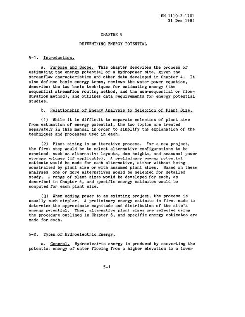
d. ~v ~ Energy generated in excess of a project or
system’s firm energy output is defined as secondary energy. Thus, it
is produced in years outside of the critical period and is often
concentrated primarily in the high runoff season of those years.
Secondary energy is generally expressed as an annual average value and
can be computed as the difference between annual firm energy and
average annual energy. Figure 5-1 shows monthly energy output for a
typical hydro project for the critical period and for an average water
year. The unshaded areas represent the secondary energy production in
an average water year.
(1) ~Power (hD). The amount of power that a hydraulic
turbine can develop is a function of the quantity of water available,
the net hydraulic head across the turbine, and the efficiency of the
turbine. This relationship is expressed by the water power equation:
5-3

EM 1110-2-1701
31 Dec 1985
SECONDARYfl
ENERGY
1 r
GENERATIONIN
AVERAGE YEAR
{
1--1
LFIRMENERGYOUTPUT /
J F MAMJ J A SON D
MONTH
Figure 5-1. Monthly energy output of a typical hydro project
hp=—
QHet
8.815
where: hp = the theoretical horsepower available
Q= the discharge in cubic feet per second
H= the net available head in feet
= the turbine efficiency
‘t
(Eq. 5-1)
(2) ~ Equation 5-1 can also be expressed
in terms of kilowatts of electrical output:
QHe
kW=— (Eq. 5-2)
11.81
5-4

EM 111O-2-17O1
31 Dec 1985
In this equation, the turbine efficiency (et) has been replaced by the
overall efficiency (e) which is the product of the generator
efficiency (e ), and the turbine efficiency (et). For preliminary
studies, a tuFbine and generator efficiency of 80 to 85 percent is
sometimes used (see Section 5-5e). Equation 5-2 can be simplified by
incorporating an 85 percent overall efficiency as follows:
(3) ~
to energy, Equation 5-2
kW = 0.072 QH (Eq. 5-3)
In order to convert a projectts Wwer output
must be integrated over time.
1
t=n
kWh = — QtHtedt
11.81 ~=o
\
(Eq. 5-4)
The integration process is accomplished using either the sequential
streamflow routing procedure or by flow-duration curve analysis.
Following is a brief description of the sources of the parameters that
make up the water power equation.
b. M The values used for discharge in the water power
equation would be the flows that are available for pwer generation.
Where the sequential streamflow routing method is used to compute
energy, discrete flows must be used for each time increment in the
period being studied. In a non-sequential analysis, the series of
expected flows are represented by a flow-duration curve. In either
case, the streamflow used must represent the usable flow available for
power generation. This usable flow must reflect at-site or upstream
storage regulation; leakage and other losses; non-~wer water usage
for fish passage, lockage, etc; and limitations imposed by turbine
characteristics (minimum and maximum discharges and minimum and
maximum allowable heads). The basic sources of flow data are
described in Chapter 4.
C* u
(1) Gross or static head is determined by subtracting the
water surface elevation at the tailwater of the powerhouse from the
water surface elevation of the forebay (Figure 5-2). At most
hydropower projects, the forebay and tailwater elevations do not
remain constant, so the head will vary with project operation. For
run-of-river projects, the forebay elevation may be essentially
constant, but at storage projects the elevation may vary as the
reservoir is regulated to meet hydropower and other discharge
requirements.
discharge, the
Tailwater elevation is a function of the total project
outlet channel geometry, and backwater effects and is
5-5

EM 111O-2-17O1
31 Dec 1985
represented either by a tailwater rating curve or a constant elevation
based on the weighted average tailwater elevation or on ‘block loadedn
operation (see Section 5-6g).
(2) Net head represents the actual head available for wwer
generation and should be used in calculating energy. Head losses due
to intake structures, penstocks, and outlet works are deducted from
the gross head to establish the net head. Information on estimating
head loss is presented in Section 5-61.
(3) A hydraulic turbine can only operate over a limited head
range (the ratio of minimum head to maximum head should not exceed
50 percent in the case of a Francis turbine, for exawple) and this
characteristic should also be reflected in power studies (see Sections
5-5c and 5-6i).
d. XficiencvL The efficiency term used in the water power
equation represents the combined efficiencies of the turbine and
generator (and in some cases, speed increasers). Section 5-5e
provides information on estimating overall efficiency for power
studies.
.
5-4. ral ADDroaches to ~st~e F@r~v=
a. utroductio~ Two basic approaches are used in determining
the energy potential of a hydropower site: (a) the non-sequential or
flow-duration curve method, and (b) the sequential streaflow routing
HEAD
LOSSES
NET
HEAD
A
_l__
GROSS
HEAD
TAlLWATER
ELEVATION
f v
—
0 .’
/’~/
[///\\Y
Figure 5-2. Gross head vs. net head
5-6
FOREBAY
ELEVATION
—

EM 1110-2-1701
31 Dec 1985
(SSR) method. In addition, there is the hybrid method, which combines
features of the SSR and flow duration curve methods.
b. Jlow-Duration Curve Method.
(1) The flow-duration curve method uses a duration curve
developed from observed or estimated streamflow conditions as the
starting point. Streamflows corres~nding to selected percent
exceedance values are applied to the water power equation (Equation 5-
2) to obtain a power-duration curve. Forebay and tailwater elevations
must be assumed to be constant or to vary with discharge, and thus the
effects of storage operation at reservoir projects cannot be taken
into account. A fixed average efficiency value or a value that varies
with discharge may be used. When specific ~wer installations are
being examined, operating characteristics such as minimum single unit
turbine discharge, minimum turbine operating head, and generator
installed capacity are applied to limit generation to that which can
actually be produced by that installation. The area under the powerduration
curve provides an estimate of the plantts energy output.
(2) This method has the advantage of being relatively simple and
fast, once the basic flow-duration curve has been developed, and thus
it can be used economically for computing power output using daily
streamflow data. The disadvantages are that it cannot accurately
simulate the use of power storage to increase energy output, it cannot
handle projects where head (i.e. forebay elevation and/or tailwater
elevation) varies independently of flow, and it cannot be used to
analyze systems of projects.
5-7 ●
(3) The flow-duration method is described in detail in Section
c* Stre~ ROUtinQ (SSR) Method< (1) With the sequential streamflow routing method, the energy
output is computed sequentially for each interval in the period of
analysis. The method uses the continuity equation to route stremflow
through the project, and thus it accounts for the variations in
reservoir elevation resulting from reservoir regulation. This method
can be used to simulate reservoir operation for hydropower
non-power objectives, such as flood control, water supply,
irrigation.
as well as
and
(2) The advantages of SSR are that it can be used to examine
projects where head varies independently of streamflow, it can be used
to model the effects of reservoir regulation for hydrofiwer and/or
other project purpses, and it can be used to investigate projects
that are operated as a part of a system. The primary disadvantage of
5-7

EM 1110-2-1701
31 Dec 1985
SSR is its complexity. Because of the large amount
required to do daily studies for long time periods,
routings are based on weekly or monthly intervals.
of weekly or monthly average flows is satisfactory.
of computer time
most sequential
Generally, the use
Where using
weekly or mnthly intervals results in an energy estimate that is
substantially in error (see Section 5-6b(4)), SSR studies should be
made using daily flows for all or part of the period of analysis.
(3) The sequential streamflow routing method is described in
Sections 5-8 through 5-14.
d. flvbrid~ The hybrid method combines features of bth
the duration curve and SSR methods. Historical streamflow and
reservoir elevation data for the period of record are obtained either
from historical records or from an existing SSR analysis (such as an
operational study performed for evaluating existing project
functions). Power output is computed sequentially for each interval
in the period of record, and the resulting data is compiled into
duration curve format for further evaluation. The hybrid method was
developed primarily to investigate the addition of power at existing
projects where head varies independently of flow. This includes flood
control storage projects and projects with conservation storage
regulated for non-power purposes. The hybrid method is usually faster
than an SSR routing but slower than the flow-duration curve method.
The hybrid method is described in Section 5-15.
(1) ~ For very preliminary or screening studies, the
flow-duration method can be used for almost any project, although
energy estimates for projects with storage or where head varies
independently of flow must be viewed with caution. Following is a
discussion of the methods that would normally be used for the various
types of projects.
(2) aun-of-mer Pro~ For the typical run-of-river
project, where head is essentially fixed (high head projects) or where
head varies with discharge (low head projects), the flow-duration
method is generally the best choice. Where head varies independently
of flow, the hybrid method should be used. SSR can also be used, but
is usually not selected for single projects because the daily flow
analysis required to get accurate results for run-of-river projects is
usually too time consuming. However, it is often desirable to use SSR
to analyze run-of-river projects that are operated as a part of a
system which also includes storage projects. An alternative to the
latter would be to use streamflows from an existing system SSR study
as input for a flow-duration or hybrid analysis.
5-8

EM 1110-2-1701
31 Dec 1985
(3) ~~e Pro.1~ SSR is the only viable method for
evaluating storage projects regulated for ~wer or for multiple
purposes including power. SSR would also normally be used for
examining the feasibility of including power at new flood control
projects or projects having conservation storage regulated for
purposes other than power. The hybrid method can be used to examine
the addition of power to an existing non-power storage project, if an
adequate historical record exists and regulation procedures are not
expected to change in the future. Otherwise, an SSR analysis must be
made.
(4) ~ Pro- Two types of studies are made in
evaluating peaking projects: hourly operation studies and period-ofrecord
studies based on longer time intervals. The power output of a
peaking project must be delivered in the peak demand hours of the day
(and of the week). Hourly operational studies are required to test
the adequacy of pondage (daily/weekly storage) to support a peaking
operation, and to evaluate the impacts of peaking operation on the
river downstream. These problems, which are dealt with in more detail
in Sections 6-8 and 6-9, require hourly SSR routings for analysis.
These hourly routings should be made for selected weeks which are
representative of the full range of expected streamflow, power demand,
and other conditions. From these studies, it is possible to determine
the level of peaking capacity that can be maintained at different flow
levels. Period-of-record power studies would be made to determine the
projectts average annual energy output, and the method used would
depend on the type of project as described in paragraphs (2) and (3)
above. The results of the hourly studies would then be applied to the
period-of-record power study to determine the project~s dependable
capacity (see Section 6-7i).
(5) ~e~ The operation of off-stream
pumped-storage projects is dictated more by the needs of the ~wer
system than by hydrologic conditions. Power system models (Section
6-9f) are normally used to estimate a project’s required energy output
However, hourly SSR routings are required to test adequacy of pondage
and impact on non-power project and river uses. Where the lower
reservoir is a storage project, period-of-record studies using the
hybrid or SSR method may be required to determine the effect of
storage regulation on the pumped-storage project’s operating head.
(6) ~ Analysis of pump-back projects (onstream
pumped-storage projects) also requires hourly SSR routing to
define ~wer operation, adequacy of pondage, and non-power impacts.
Identification of the peak demand seasons and determination of the
frequency of pumped-storage operation would be made using power system
models, and this data would be used in conjunction with period-of-
5-9

EM 1110-2-1701
31 Dec 1985
record SSR routings to estimate annual energy output and dependable
capacity (see Section 7-6).
(7) &stem Studies. Where a project is operated as a part of a
system, SSR analysis is required to properly model the impact of
system operation on that project’s power output. The only case where
the flow-duration or hybrid method might be used would be in the
examination of a single existing project with no power storage, where
an adequate historical record exists, no changes in project operation
are expected, and no changes in streamflow resulting from the
regulation of upstream projects are expected.
5-5. ine Character~
a. &ner& Certain turbine characteristics, such as efficiency,
usable head range, and minimum discharge, can have an effect on
a hydro project’s energy output. For preliminary ~wer studies, it is
usually sufficient to use a fixed efficiency value and ignore the
minimum discharge constraint and possible head range limitations.
However, for a feasibility level study, these characteristics should
be accounted for in cases where they would have a significant impact
on the results. This section presents some general information on the
turbine characteristics required for making power studies and on the
operating parameters involved in the selection of a specific turbine
design.
(1) A variety of turbine types are available, each of which is
designed to operate in a particular head and flow range. Figure 2-35
illustrates the normal operating ranges for each type. In addition, a
specific turbine is capable of operating within a limited head range.
A horizontal Kaplan unit, for example, has a ratio of maximum head to
minimum head of about 3 to 1. Table 5-1 (Section 5-6i) describes the
usable operating head range for each of the major turbine types.
(2) Where possible, a runner design is selected such that the
turbine can operate satisfactorily over the entire range of expected
heads. This is especially important in the case of storage projects,
where drawdown characteristics may be a major factor in selection of
the type of turbine to be installed. At storage projects with a wide
head range, it is sometimes possible to utilize interchangeable
runners in order to ❑aintain generation over the full head range.
(3) When adding power facilities to projects not originally
designed for power operation, head ranges may exceed the capabilities
of any turbine type. Examples are (a) low head projects where the
5-1o

EM 1110-2-1701
31 Dec 1985
tailwater elevation is so high at high discharges that the head falls
below the turbinels minimum head and the project ‘drowns outn, and
(b) new power installations at existing storage projects, where the
range of head experienced in normal project operation exceeds the
capabilities of a single turbine runner.
(4) In preliminary studies, it is not necessary to account for
limitations on the turbine usable head range. However, they should be
accounted for in feasibility level studies. This is done by
specifying maximum and minimum operating heads in the power study.
When making the routing (or duration curve analysis), no generation is
permitted in those periods when the head falls outside of this range.
(1) Design head is defined as the head at which the turbine will
operate at best efficiency. The planner determines the head at which
best efficiency is desired from the power studies and provides this
value to the hydraulic machinery specialist for selection of an
appropriate turbine design. Since it is usually desirable to obtain
best efficiency in the head range where the project will operate most
of the time, the design head is normally specified at or near average
head. However, the design head should also be selected so that the
desired range of operating heads is within the permissible operating
range of the turbine.
(2) For single-purpose power storage projects, a preliminary
estimate of average head can be obtained by determining the net head
at the reservoir elevation where 25 percent of the power storage has
been drafted. For multiple-purpose storage projects, including flood
control and power, average head can be based on a draft of 33 to 50
percent. A more refined value of average head can be derived by
averaging the heads computed for each interval in the period-of-record
power routing studies. In some cases it is desirable to develop a
weighted average head, with the head values for each period weighted
by the corresponding power discharge.
(3) For run-of-river projects, design head can be determined
from a head-duration curve by identifying the midpoint of the head
range where the project is generating ~wer (Figure 5-3). Design head
would normally be based on operation over the entire year, but where
dependable capacity is particularly important, it may be desirable to
base it on operation in the peak demand months only. For pondage
projects which operate primarily for peaking, design head is often
based on a weighted average head, which is weighted by the amount of
generation at each head.
5-11

EM 1110-2-1701
31 Dec 1985
z (head x generation)
Weighted average head = (Eq. 5-5)
~ (generation)
This analysis would be based on hourly routing studies. Because
period-of-record hourly studies are not practical, the analysis would
have to be limited to a sufficient number of weeks to be
representative of the period of record.
(4) Rated head is defined as
obtained with turbine wicket gates
minimum head at which rated output
20
1 18- _ ———MAXIMUM HEAD
16-
14-
+
Lu
y 12z
E
< lo-
Lll
1
+
: 8--
1
that head where rated pwer is
fully opened. Thus, it is the
can be obtained. A generator is
——–DESIGNHEAD
MINIMUM HEAD
6- 1
— 460/o — —
460/o —
I
4-
2-
‘1 I
0 I I I 1 I I I I I
0 10 20 30 40 50 60 70 80 90 100
PERCENTOFTIME EQUALEDOREXCEEDED
Figure 5-3. Head-duration curve for run-of-river
project, showing how design head can be determined
5-12

EM 111O-2-17O1
31 Dec 1985
selected with a rated capacity to match the rated power output of the
turbine at a specific power factor (usually 0.95 for large synchronous
generators). Above rated head, the generator capacity limits pwer
output, so the unit?s full rated capacity can be obtained at all heads
above rated head. Below rated head, the maximum achievable power
output with turbine gates fully open is less than rated capacity
(Figure 5-4).
(5) The selection of rated head is generally a compromise based
on cost, efficiency, and dependable capacity considerations. At some
projects, the range of head experienced in normal operation is small
enough that a unit can be selected such that rated output can be
i=
w L
c1
$
x
MAXIMUM ALLOWABLE HEADOFTURBINE
.—— ———.— ——.— ——. ~.__—–——
.—— —— —— —— ——
RATED HEAD
@p/
_f__
/’
/
/
.7––––7–7—
/ /
4 / /’
,// /
/ //
//
/ /’ ‘/
‘/
/’GENERATOR ./ * ‘/
LIMIT /’
/’ /
/’
/ / /
+–– ___
/ /’ ,’
/’ // //
/
/ /
/’ /’
CAPACITY
BLEHEADOFTURBINE
.—— ——— —.—. ——— —
Figure 5-4. Turbine performance curve for a specific design
(solid line represents maximum output of unit)
5-13

EM 1110-2-1701
31 Dec 1985
obtained over the entire operating range if desired (Figure 5-5). At
other projects, the head range is such that the operating head drops
below the rated head under some operating conditions, with a resulting
decrease in generating capability. Examples of the latter are (a) a
storage project with a large drawdown, where head drops below rated
head at low pool elevations (Figure 5-6), and (b) a pondage project
with a large installed capacity, where the tailwater encroachment at
high plant discharges causes head to fall below rated head. Figure
5-7 illustrates a capacity versus discharge curve for various numbers
of 5 megawatt units at a low head run-of-river project. This figure
shows how output can drop off at the higher discharge levels due to
tailwater encroachment.
MAXIMUM ALLOWABLE HEADOFTU7RBINE
——. -— — ————— — ——— — — —-—— —-— —
.-_— -
PROJECT OPERATING
HEAD RANGE
/
/
/
––_–__.r_7_
/ GENER~~TO~ /’ //
/
~
/ -/
CAPACITY
Figure 5-5. Turbine design from Figure 5-4 as applied
to a project with a narrow operating head range
5-14

(6) It is difficult to generalize about the
between rated head and design head, because it is
type of turbine and how the project is operated.
EM 1110-2-1701
31 Dec 1985
relationship
a function of the
However, there are
some overall guidelines that may prove helpful. It is not usually
cost-effective to select a rated head equal to the expected maximum or
minimum head, because this would result in either an oversized turbine
or oversized generator, respectively (see Section 5-5g). The only
exception would be where the ratio of drawdown to maximum head is
small (Figure 5-5), in which case the rated head might be equal to the
minimum head.
CAPACITY
Figure 5-6. Turbine design from Figure 5-4 as applied
to a storage project with large operating head range
5-15

EM 1110-2-1701
31 Dec 1985
(7) For a pure run-of-river project, the rated head is usually
defined by the maximum plant discharge (hydraulic capacity). For
example, a flow-duration curve would be examined, and one or more
discharges would be selected for detailed study. For each
alternative, the net streamflow available for power generation would
be determined, and this would define the hydraulic capacity for that
plant size. The net head available at the streamflow upon which the
hydraulic capacity is based would be the rated head. The design head
for this type of project would typically be based on the midpoint of
the head range where the plant is generating power, and this would
usually be higher than the rated head (see Figure 5-19).
(8) For projects with seasonal storage, it is usually desirable
to obtain rated output over a range of heads. Hence, the rated head
would typically be lower than the design head (the average head). For
preliminary studies, a rated head equal to or slightly below (95
percent of) the estimated average head can usually be assumed. For
more advanced studies, the rated head should be defined more specifi-
1 2 3 45 6
DISCHARGE-1OOO CFS
Figure 5-7. Capacity vs. discharge for run-of-river
project for alternative plant sizes
5-16

EM 1110-2-1701
31 Dec 1985
tally. For a storage project, the design head could be estimated from
the initial period-of-record sequential routings, as described in
paragraph (2), above. The head range in which it is desired to obtain
rated head could be defined by examining the routing in the light of
power marketing considerations. For example, in systems where
dependable capacity is important, it would be desirable to obtain
rated capacity throughout the normal range of drawdown during the peak
demand ❑onths. With this information, the hydraulic machinery
specialist would select a turbine design that most closely meets these
requirements, thereby defining the rated head. Head-duration curves
are very helpful in selecting the rated head.
(9) Run-of-river projects with pondage would generally be
treated similarly to storage projects, in that a turbine design would
be selected which permits operation at a good efficiency level most of
the time while permitting the delivery of rated output over the head
range where the project operates most of the time. At some projects,
the ratio of drawdown to maximum head is such that rated head can be
delivered through the entire operating range (as in Figure 5-5).
Hourly operation studies are often required to properly define the
operating head range, and this would include the head range where the
plant is expected to operate most of the time, as well as the extremes
(see paragraph (3) and section 6-9).
(10) Hydraulic capacity was mentioned as a key parameter in
rating run-of-river projects, and it is important in rating projects
with load-following capability as well. For multiple-unit plants,
the units would normally be rated at the condition where all of the
units in the plant are assumed to be operating at full gate discharge
(i.e., with the plant operating at hydraulic capacity). The rated
discharge of individual units would be the desired plant hydraulic
capacity divided by the number of units. The rated head would be
based on the tailwater conditions corresponding to the total plantvs
hydraulic capacity, and not the tailwater elevation corresponding to a
single unit operating at full gate discharge. Further information on
selection of hydraulic capacity (plant size) for peaking projects can
be found in Section 6-6d.
(11) Rated head is the minimum head at which the turbine manufacturer
must guarantee rated output. However, turbines are sometimes
able to deliver rated capacity at heads below rated head,
because the manufacturers typically build some cushion into their
designs to insure that they meet specifications. The minimum head at
which a specific turbine can actually deliver rated capacity is called
the critical head. Although the term critical head is sometimes used
synonymously with rated head, to be precise, a projectts critical head
cannot be identified until the turbines have been purchased and
5-17

EM 1110-2-1701
31 Dec 1985
tested. Therefore, only the term rated head should be used in
planning and design studies.
(1) Cavitation and vibration problems limit turbines to a
minimum discharge of 30 to 50 percent of rated discharge (rated
discharge being discharge at rated head with wicket gates fully open).
This characteristic should be accounted for in power studies, and it
may in some cases influence the size and number of units to be
installed at a given site. For example, if a minimum downstream
release is to be maintained at a storage or pondage project for nonpower
purposes, and it is desired to maintain power production during
these periods, a unit must be selected which is capable of generating
at the required minimum discharge. For run-of-river projects, proper
accounting for minimum discharge is equally important. Streamflows
below the single-unit minimum discharge will be spilled, so flowduration
curves should be examined carefully to determine the size and
number of units that will best develop the energy potential of a given
site. The example in Section 6-6g illustrates the impact of singleunit
minimum turbine discharge on a project’s energy output.
(2) In preliminary power studies, minimum discharge can usually
be ignored, but once a tentative selection of unit size or sizes has
been made, a minimum single-unit turbine discharge must be applied to
the energy computation. For more advanced studies, a minimum
discharge based on the data presented in Table 5-1 (Section 5-6i)
can be assumed. Once a specific turbine design has been selected, the
minimum discharge associated with that unit should be used.
(1) The efficiency term used in power studies reflects the
combined efficiencies of the turbine and generator. Generator
efficiency is usually assumed to remain constant at 98 percent for
large units and 95 to 96 percent for units smaller than 5 ~.
However, turbine efficiency varies with the operational parameters of
discharge and head. The efficiency characteristics of a turbine vary
with type and size of unit and runner design. Figure 5-8 shows
typical performance curves for a Francis turbine.
(2) In reconnaissance level power studies, a fixed efficiency of
80 to 85 percent may be used to represent the combined efficiency of
the turbines and generators. A value of 85 percent can be applied to
installations where the larger custom-built turbines would be used.
The smaller standardized Francis and tubular turbines and units
requiring gearboxes have lower efficiencies, and an overall efficiency
of 80 percent should be used for reconnaissance studies of projects
5-18

EM 1110-2-1701
31 Dec 1985
where this type of units would installed. In feasibility studies, it
is necessary to look at the specific characteristics of the type of
units being considered and the range of heads and flows under which
they will operate to determine the appropriate efficiency value or
values to use.
(3) Figure 2-36 shows that each turbine has a range of head and
flow where efficiency remains relatively constant. Outside of this
range, efficiency drops off rapidly. This characteristic is most
apparent with units such as Francis and fixed blade propeller
turbines. In power studies where the head and flow are expected to
lie within the range of relatively constant efficiency, an average
efficiency value can be used. However, where the units are expected
to operate over a wide range of flows and/or head, an efficiency curve
should be used instead of a fixed value.
60 o
‘“T
I MINIM
.—— —
MUM H-D> I I
20 40 60 80 100 120
PERCENT DISCHARGE
Figure 5-8. Typical Francis turbine performance curve
5-19

EM 1110-2-1701
31 Dec 1985
(4) The variation of efficiency with head can be quite
significant at storage projects with large head ranges and at low-head
run-of-river projects. %me sequential routing programs have
provisions for modeling the variation of efficiency with head, and
others can accommodatevariation with both head and discharge. Where
only variation with head is ❑odeled, values of efficiency should be
selected which are most representative of the discharge levels at
which the plant will operate. When kW/cfs curves are used (see
Appendix G), the variation of efficiency with head would be
incorporated directly in that parameter. At other types of projects,
the variation of efficiency with discharge can be an important
consideration. Section 5-6k discusses the modeling of efficiency
versus head and discharge in more detail.
(1) Turbine selection is an iterative process, with preliminary
power studies providing general information on approximate plant
capacity, expected head range, and possibly an estimated design head.
One or more preliminary turbine designs are then selected and their
operating characteristics are provided as input for the more detailed
power studies. The results of these studies make it possible to
better identify the desired operating characteristics and thus permit
final selection of the best turbine design and the best plant
configuration (size and number of units).
(2) Turbine performance data for various types of turbines is
essential to the selection process. While data can be obtained
directly from the manufacturer, it is recommended that field offices
work instead through one of the Corps Hydroelectric Design Centers.
Hydraulic machinery specialists in these offices have access to
performance data for a wide range of unit designs from various
manufacturers, and they are able to recommend runner designs that are
best suited to any given situation. Performance curves can then be
provided to the field office for the selected turbine design.
(3) In preparing a request to a Hydroelectric Design Center for
turbine selection, the following information should be provided.
. expected head range
. head-duration data (not required but very useful)
● design head (optional)
. total plant capacity (either hydraulic capacity in cfs or
generator installed capacity in megawatts)
● minimum discharge at which generation is desired
. alternative combinations of size and number of units to be
considered (optional)
5-20

EM 1110-2-1701
31 Dec 1985
. head range at which full rated capacity should be provided
if pssible (optional)
● tailwater rating curve
(1) The rated output of a generator is chosen to match the
output of the turbine at rated head and discharge. As was discussed
earlier, the head at which the turbine is rated can vary depending on
the type of operation as well as economics. An example will serve to
illustrate some of the trade-offs involved in selecting this rating
point.
(2) Assume that a power installation is being considered for a
multiple-purpose storage project which is operated on an annual
drawdown cycle, similar to that shown in Figure 5-12. The maximum
head (head at full pool) is 625 feet, and the minimum head (head at
minimum Pol) is 325 feet. From the initial sequential routing
studies, the average head is found to be 500 feet, and that head is
used as the design head (head at which best efficiency is desired).
It is proposed to investigate a plant which is capable of passing 1000
cfs at the design head.
(3) Assume that the turbine selection procedure outlined in
Section 5-5f is followed, and it is found that a Francis turbine of
the design shown in Figure 5-8 provides suitable performance for the
specified range of operating conditions. Applying this turbine to
these operating conditions, the performance curve shown as Case 2 on
Figure 5-9 is obtained.
(4) Rating the unit at three different heads will be considered:
design head, maximum head, and minimum head. These are not the only
options available. They could be rated at any intermediate head as
well, but examining these three alternatives will illustrate some of
the factors involved in selecting the conditions for rating a
generating unit.
(5) Consider first rating the unit at the design head. This
would be a reasonable alternative to consider for rating units at a
project with a head range of this magnitude. Case 1 on Figure 5-9
shows the performance characteristics of such a unit. The turbine
would be rated to produce 36.0 megawatts at a head of 500 feet and a
full-gate discharge of 1000 cfs. A generator of the same 36.o megawatt
rated output would be specified. Note that the turbine would
actually be rated in terms of its horsepwer output, but to simplify
the discussion, its equivalent megawatt output will be used. The
dashed line shows additional capability of the turbine which is not
realized because of the limit imposed by the 36.O megawatt generator.
5-21

EM 1110-2-1701
31 Dec 1985
t
I
I
1 1 1 1 r 1 I 1 1 I
o~
c1 10 20 30 40 50
CAPACITY (MEGAWATTS)
CASE2: RATED AT MAXIMUM HEAD RATING POINT)
o 10 40 50
CAP::ITY (MEGAW3iTTS)
Figure 5-9. Alternative rating points for a given Francis
turbine design applied to a given storage project
5-22

~ CASE 3: RATED AT MINIMUM HEAD
I
//’
EM 1110-2-1701
31 Dec 1985
-—7
//--- /’
RATING POINT-. _-----’
/“
/“
/’
/
//
/
/
/
/
/
/
RATED CAPACITY, = ‘
(17.5 MW)
/
/
/
/
/
/
,~’
/ /
o~ f 1 I 1 1 1 1 t
o 10 20 30 40 50
CAPACITY (MEGAWATTS)
Figure 5-9 (continued)
Figure 5-10 shows the unit characteristics as applied to Figure 5-8,
including the turbine efficiencies obtained under various operating
conditions.
(6) Next, rating the unit at maximum head will be considered.
The same turbine would be used, but in this case it will be rated to
produce 49.5 megawatts at a head of 625 feet and a discharge of 1120
cfs. A 49.5 megawatt generator would also be specified (Case 2 on
Figures 5-9 and 5-10). Rating the unit in this manner will insure
that the turbinels full potential will be utilized, and that the
maximum amount of energy can be produced. The additional energy
production is realized because the unit is capable of greater output
when high heads are accompanied by high discharges. However, this
additional output is achieved at the expense of higher costs for the
larger generator, transformer, and associated buswork and switchgear.
In most cases, the amount of time a project would experience these
combinations of high heads and high flows is too small to justify the
additional costs, but this can be verified only through economic
analysis.
5-23
/

EM 111O-2-17O1
31 Dec 1985
700
600
550
i=
UI 500
k
400
350
‘-~” “’{”>
-———-
DESIGN
HEAD
—
.——-—- .
I
Rating Point
for Case 2
1%
MINIMUM HEAD
300 I
o 200 400 600 800 1000 1200
❑ ADDITIONAL
m ADDITIONAL
DISCHARGE (CFS)
OPERATING RANGE
FOR CASE 1
OPERATING RANGE
FOR CASE 2
Figure 5-10. The operating ranges and efficiencies for
the alternative turbine rating points shown on Figure 5-9
5-24

EM 1110-2-1701
31 Dec 1985
(7) The third option being considered is to rate the unit at
minimum head. In this case, the turbine would be rated to produce
17.5 megawatts at a head of 325 feet and a discharge of 790 cfs (Case
3 in Figures 5-9 and 5-10). Using this approach, it will be possible
to obtain the full rated output throughout the entire operating head
range, and this may be a consideration if the projectfs dependable
capacity output is of prime concern. However, it should also be noted
that the maximum discharge at the 500 foot design head is only 48o
cfs, well below the 1000 cfs requirement. To pass 1000 cfs at 500
feet of head, the unit would have to be rated to produce 36.4
megawatts at the rated head of 325 feet. This requirement could be
met by installing a larger turbine runner of the same design. The
corresponding rated discharge would be 1640 cfs. The larger unit will
be able to capture some additional energy when high discharges are
experienced in the low head range. This additional performance would
be achieved at the cost of a larger runner, a larger penstock and
spiral case, and perhaps larger intake and powerhouse structures. In
addition, it can be seen from Figure 5-10 that the unit will be
operating at relatively low efficiencies much of the time, which will
result in a lower energy output over most of the operating range
(compared to Cases 1 and 2) and which could result in rough operation
of the unit.
(8) It can be seen from the examples that matching the generator
to the turbine at either maximum head or minimum head is not usually
desirable, at least not for a project with a large operating head
range. Rating a unit at maximum head usually results in an oversized
generator and rating the unit at minimum head results in an oversized
turbine. However, the example does show the general effect of varying
the rated head on project cost and performance. When making the final
analysis of a proposed powerplant, it is common to test a range of
rated heads, as well as different turbine runner designs, using
economic analysis to select the recommended plan. However, this would
not generally be done until the project reaches the design stage. At
the planning stage, it is usually satisfactory to consider only a
single rated head, selected using the general guidelines presented in
Sections 5-5c (3) through (9), but also taking into account the
relationships described above. As with the turbine selection process,
the determination of rated head should be made in cooperation with
hydraulic machinery specialists from one of the Hydroelectric Design
Centers.
a. fitro~ This section describes the data required for
energy potential studies. The data specifically required for a given
study varies depending on the type of project and the method used for
5-25

EM 1110-2-1701
31 Dec 1985
computing the energy. This section describes each data element in
detail, and Tables 5-2, 5-3, 5-4, 5-12, and 6-2 summarize specific
data required for each of the respective types of studies.
(1) The time interval used in a power study depends on the type
of project being evaluated, the type of power operation being
examined, the degree of at-site and upstream regulation, and the other
functions served by the project or system. Longer time intervals,
such as the month, are generally preferable from the standpoint of
data handling. However, where flows and/or heads vary widely from day
to day, shorter intervals may be required to accurately estimate
energy output.
(2) A daily time interval should generally be used with the
duration curve method. Weekly or monthly average flows tend to mask
out the wide day-to-day variations that normally occur within each
week or month. As a result, the higher and lower streamflow values
are lost, and the amount of streamflow available for pwer generation
may be substantially overestimated (see Figure 5-29). The only case
where weekly or monthly average flows could be used would be where
storage regulation minimizes day-to-day variations in flow.
(3) The time interval used for the sequential stremflow routing
method depends on the type of project being studied. For projects
with seasonal power storage, a weekly or monthly interval is normally
used. A weekly interval would give better definition than a monthly
interval, but where a large number of projects are being regulated
over a long historical period, the monthly interval may be the most
practical choice from the standpoint of data processing requirements.
Where the monthly interval has been adopted but the hydrologic
characteristics of the basin produce distinct operational changes in
the middle of certain months, half-month intervals may be used. In
some snowmelt basins, for example, reservoir refill typically begins
in mid-April, and to model this operation accurately, Aprils are
divided into two half-month intervals.
(4) During periods of flood regulation, streamflows may vary
widely from day to day, and daily analysis may be required, both to
accurately estimate energy potential and to properly model the flood
regulation (if the routing model is being used to simultaneously do
flood routing and pwer calculations). One approach is to use a daily
or multi-hour routing during the flood season and weekly or monthly
routing during the remainder of the year. Some sequential routing
models, including HEC-5, can handle a mix of routing intervals.
5-26

EM 1110-2-1701
31 Dec 1985
(5) For SSR analysis of a run-of-river project with no upstream
storage regulation, daily flows must be used. Where seasonal storage
provides a high degree of streamflow regulation and streamflows at the
run-of-river project remain relatively constant from day to day,
weekly, hi-weekly, or monthly intervals may be used.
(6) For studies of peaking projects, pump-back projects, and
off-stream pumped-storage projects, hourly sequential routing studies
may be required (Section 6-9). These studies are generally made for
selected weeks which are representative of the total period of record.
(7) when using the hybrid method (Section 5-4d), a daily routing
interval should be used, for the same reasons as were cited for the
duration curve method.
(8) The level of study may also influence the selection of the
routing interval. In cases where daily data would be required at the
feasibility level, weekly or monthly data may be adequate for
screening or reconnaissance studies.
(1) For sequential routing studies, historical streamflow
records are normally used. The basic sources of historical streamflow
data and methods for adjusting this data for hydrologic uniformity are
described in Sections 4-3 and 4-4. To avoid biasing the results, only
complete years should be used.
(2) Historical records are frequently used for flow-duration and
hybrid method analyses also. However, the data must be consistent
with respect to upstrem regulation and diversion. In some cases,
period-of-record sequential routing studies have previously been
performed for the pur~ses of analyzing flood control operation or
other project functions. Since these routings would already reflect
actual operating criteria and other hydrologic adjustments, they
should be used when they are available.
(3) For hourly studies, flow is usually obtained from the weekly
or monthly period-of-record sequential routing studies that describe
the long-term operation of the project being studied.
(1) Thirty years of historical streamflow data is generally
considered to be the minimum necessary to assure statistical
reliability. However, for many sites, considerably less than 30
years of record is available. Where a shorter record exists, several
alternatives for increasing data reliability are available.
5-27

EM 1110-2-1701
31 Dec 1985
(2) For a large project, particularly one with seasonal storage,
the stremflow record should be extended using correlation techniques,
basin rainfall-runoff models, or stochastic streamflow generation
procedures (Section 4-3d).
(3) For small projects where energy potential is to be estimated
using the flow-duration method, correlation techniques can also be
used. A short-term daily flow-duration curve can be modified to
reflect a longer period of record by correlating the streamflow with
nearby long-term gaging stations.
(4) For small projects where sequential streamflow routing is
to be used, and less than 30 years of flow data are available, the
record should be tested by comparing with other nearby gaging stations
to determine if it is representative of the long term. If so, the
analysis could be based on the available record, but, if not, the
record should be extended using one of the methods outlined in Section
4-3d.
(5) In examining the addition of power to an existing flood
control storage project, the period of record for regulated project
outflows may be relatively short, but a long term record of unregulated
flows usually exists. If the available record of regulated
flows is not representative of the long term, regulated flows for
the entire period of record could be developed using a reservoir
regulation model such as HEC-5 or SSARR.
(6) When evaluating a project with seasonal power storage (or
conservation storage for multiple purposes including power), care
should be taken to insure that the streamflow record includes an
adverse sequence of streamflows having a recurrence interval suitable
for properly analyzing the projectts firm yield (say once in 50
years). This could be tested by comparing the available record with
longer-term records from other gages or by analyzing basin precipitation
records. If the available sequence does not include an
adverse flow sequence suitable for reservoir yield analysis, it should
be extended to include one.
(7) The discussion in the preceding paragraphs applies primarily
to feasibility and other advanced studies. For reconnaissance
studies, extensive hydrologic analysis can seldom be justified. An
estimate of the projectls energy output can be developed using the
available record, and an approximate adjustment can be made if
necessary to reflect longer term conditions.
5-28

EM 1110-2-1701
31 Dec 1985
(1) Not all of the streamflow passing a dam site may be
available for power generation. Following is a list of some of the
more common streamflow losses. The consumptive losses include:
. reservoir surface evaporation losses
● diversions for irrigation or water supply
The non-consumptive losses include:
● navigation lock requirements
. requirements of fish passage facilities
. other project water requirements
● leakage through or around dam and other embankment
structures
. leakage around spillway or regulating outlet gates
. leakage through turbine wicket gates
(2) Techniques for estimating each of these losses are discussed
in Section 4-5h. Losses may be assumed to be uniform the year around,
or they can be specified on a mnthly or seasonal basis. If the
streamflow is to be routed to downstream projects or control points,
it will be necessary to segregate the losses into consumptive and
nonconsumptive categories. Otherwise, they can be aggregated into a
single value for each period (or the year if no seasonal variation is
assumed). As noted in Section 4-5h, evaporation losses at storage
projects are treated as a function of surface area (and hence
reservoir elevation).
(3) When examining the addition of power to an existing project,
it is common to use either a historical record of project releases of
an existing period-of-record sequential routing study. This data
usually reflects consumptive losses already.
f. Cs ●
(1) In sequential streamflow routing studies, the type of
reservoir data that must be provided depends on the type of project
being examined. For storage projects, this would include storage
volume versus reservoir elevation data, and (where evaporation losses
are treated as a function of reservoir surface area) surface area
versus elevation data. Examples of storage-elevation and areaelevation
curves are shown in Section 4-5c. Where physical or
operating limits exist, maximum and/or minimum reservoir elevations
would also be identified.
5-29

EM 1110-2-1701
31 Dec 1985
(2) For some run-of-river projects, a constant reservoir
elevation can be specified, but for others, it may be necessary to
develop a forebay elevation versus discharge curve. For run-of-river
projects with pondage, reservoir elevation will vary from hour to
hour, and the average daily elevation may vary from day to day. In
the hourly modeling of peaking operations, this variation in elevation
must be accounted for, and storage-elevation data must be provided in
the model. However, when these proJects are being evaluated for
energy ~tential, and daily, weekly, or monthly time intervals are
being used, an average pool elevation should be specified. The
average elevation can be estimated from hourly operation studies, and
it may be specified as a single value or as varying seasonally (for
example, assume a full pool in the high flow season and an average
drawdown during the remainder of the year).
(3) When using the flow-duration method, either a fixed
(average) reservoir eleVatiOn or an elevation versus discharge
relationship must be assumed for all types of projects. When using
the hybrid methodg reservoir elevations are obtained for each interval
from the historical record or from a base sequential streamflow
routing study.
(1) Three basic types of tailwater data may be provided:
. a tailwater rating curve
● a weighted average or ‘block-loadedW tailwater elevation
● elevation of a downstream reservoir
(2) For most run-of-river projects or projects with relatively
constant daily releases, a tailwater rating curve would be used. At
peaking projects, the plant may typically operate at or near full
output for part of the day and at zero or some minimum output during
the remainder of the day. In these cases, the tailwater elevation
when generating may be virtually independent of the average
streamflow, except perhaps during periods of high runoff. For
projects of this type, a single tailwater elevation based on the
peaking discharge is often specified. It could be a weighted average
tailwater elevation, developed from hourly operation studies and
weighted proportionally to the amount of generation produced in each
hour of the period examined. In other cases, it might be appropriate
to use a ‘block-loadedW tailwater elevation, based on an assumed
typical output level (Figure 4-7).
(3) There is sometimes a situation where a downstream reservoir
encroaches upon the project being studied: i.e., the project being
studied discharges into a downstream reservoir instead of into an open
5-30

EM 111O-2-17O1
31 Dec 1985
river reach. This encroachment may be in effect all of the time or
just part of the time. During periods when encroachment occurs, the
project tailwater elevation should be based on the elevation of the
downstream reservoir.
(4) In some cases, two or more different tailwater situations
may exist at a single project during the course of the year. It may
operate as a peaking project most of the year, and during this period
a ‘block-loadedW tailwater elevation may be most representative.
During the high flow season, the tailwater rating curve may best
describe the projectts tailwater characteristics. Some energy models
provide all three tailwater characteristics (rating curve, weighted
average or block-loaded elevation, and elevation of downstream
reservoir) and select the highest of the three fok each interval.
(5) when SSR modeling is done on an hourly basis, it is
necessary to reflect the dynamic variation of tailwater during peaking
operations (i.e., the fact that the tailwater elevation response lags
changes in discharge). A simple lag of the streamflow hydrographymay
be applied to reflect the time required for tailwater to adjust to
changes in discharges, or more sophisticated routing techniques may be
applied, Section 4-5b provides additioml information on developing
tailwater data.
(1) The powerplant installed capacity establishes an upper limit
on the amount of energy that can be generated in a period. Installed
capacity is one of the variables considered in evaluating a hydro
project, and it is common to make energy estimates for several
alternative plant sizes. However, when other variables, such as dam
height, storage volume, and project layout are being considered as
well, a systematic approach is needed to minimize the number of power
studies made. A frequently used procedure Is to assume a common plant
sizing parameter for all project configurations, one which results in
most of the energy being captured. This parameter could be a typical
plant factor or, in the case of a duration curve analysis, a specific
point on the flow-duration curve. Then, once the range of possible
project configurations has been screened down to one or more most
likely candidates, alternative plant sizes would be tested.
(2) For preliminary studies, energy estimates are sometimes made
without applying an installed capacity constraint. The resulting
value, which represents the total energy potential of the site, can be
used to select a range of plant sizes for more detailed study.
(3) Formerly, plant capacity was specified in terms of both a
rated or nameplate capacity and a somewhat higher overload capacity
5-31

EM 111O-2-17O1
31 Dec 1985
(usually 115 percent of nameplate). At the present time, only a
single rated capacity value is specified, and this value includes
overload characteristics (see Section 6-lb). Chapter 6 gives
additional information on plant size selection.
(1) Maximum and minimum turbine discharge and the turbine~s
usable head range establish limits on the amount of energy that can be
developed at a site. In making energy computations, it is necessary
to check to insure that the net head and usable discharge values for
each time interval fall within the allowable range for the type of
turbines being considered, so these values must be identified.
Sections 2-6 and 5-5 provide general information on turbine characteristics
and turbine selection. Following is some specific data on
discharge and head ranges for the various types of turbines.
(2) In planning studies, plant size is often specified initially
in terms of hydraulic capacity. The hydraulic capacity would also be
the plant~s maximum discharge, and in most cases can be assumed to be
the same as the plant’s rated discharge (see Section 6-lb(8)). The
maximum (or rated) discharge of individual units would be defined by
the number and size of the units (see Section 6-6f).
(3) Cavitation problems and the possibility of rough operation
preclude generation below a minimum discharge (see Section 5-5d), and
the minimum discharge for a single unit establishes the plant?s
minimum allowable power discharge. Table 5-1 lists factors for
computing minimum discharges for different types of turbines given a
units rated discharge. These values can be used for initial power
studies, but once a unit design has been selected, the specific
minimum discharge characteristics of that unit should be used.
(4) Likewise, a turbine is only capable of operating
satisfactorily over a limited head range (Section 5-5b)~ and this
should be reflected in energy studies. For preliminary studies, the
maximum head ranges listed in Table 5-1 should be used. These ranges
are only approximate. Once a unit design has been selected, the
specific head range characteristics of that unit should be used
instead.
Je Wlcfs Curve. When hand routing techniques and certain
computer programs are used to evaluate the energy output of a storage
project, kW/cfs versus elevation and kW/cfs versus head curves are
sometimes used to simplify the analysis. These curves account for the
variation of powerplant efficiency with head, and the kW/cfs versus
elevation curves account for head loss and tailwater elevation as
5-32

EM 111O-2-17O1
31 Dec 1985
TABLE 5-1
Discharge and Head Ranges for Different Types of Turbines
Ratio of Minimum Ratio of Minimum
Discharge to Head to
ine TvDe &ted D~ Heti
Francis 0.40 0.50
Vertical shaft Kaplan 0.40 0.40
Horizontal shaft Kaplan 0.35 0.33
Fixed blade propeller 0.65 0.40
Fixed gate adjustable
blade propeller 0.50 0.40
Fixed geometry units
(pumps as turbines) 0.80
Pelton (adjustable
nozzles) 0.20 0.80
well. Appendix G describes how kW/cfs curves can be developed and
used.
k.
MficiencvL
(1) The efficiency of turbine-generator units varies with both
head and discharge and with turbine type. Section 5-5e describes
these efficiency-characteristicsin some detail. The following
paragraphs summarize how efficiency should be treated for different
types of projects and studies.
(2.) For preliminary studies, it is common to assume a fixed
overall efficiency of 80 to 85 percent.
(3) A fixed efficiency value can also be used for feasibility
level studies of small hydro projects where the head fluctuation is
small compared to total head (less than 10 percent). A value of 80 to
85 percent can be used prior to turbine selection, but once a
turbine design has been chosen, an average efficiency based on the
characteristics of that unit should be used.
(4) For feasibility studies of large projects, or small projects
where large head fluctuations are experienced, the variation of
efficiency can have a significant effect on energy output. For small,
5-33

EM 111O-2-17(.)]
31 Dec 1985
low-head projects, where head varies directly with discharge, an
efficiency versus discharge relationship can be derived (see Section
5-7n).
(5) For projects where head varies independently of discharge,
an efficiency versus discharge curve can be used if head does not vary
substantially. Where head does vary substantially, several alternatives
are available. For projects with four or more units, there is
considerable flexibility of operation. The number of units that are
placed on-line at any given discharge would be selected such that they
would all be operating at or near the point of best efficiency for the
given discharge. In these cases, an efficiency versus head curve can
be developed. Figure 5-11 shows an efficiency vs. head curve for a
multiple-unit Francis installation. This curve was developed from the
turbine performance curve shown on Figure 5-8, based on the units
operating at the Pint of best efficiency at each head. The
efficiency values from Figure 5-8 were reduced by an additional two
percent to account for generator losses. Where a project is normally
“block loaded” (see Figure 5-10, the plant would always operate at or
NETHEAD (FEET)
Figure 5-11. Net head vs. efficiency curve
for Francis turbine (multiple-unit installation)
5-34

EM 1110-2-1701
31 Dec 1985
near full plant output. An efficiency versus head curve could be
developed for this type of project as well.
(6) Where it is considered necessary to model the variation of
efficiency with both head and discharge, several techniques are
available. One example is the procedure used in North Pacific
Division~s HYSSR model (see Appendix C), where three efficiency versus
head curves are used:
. operation at best efficiency
● operation at full gate discharge
● operation at rated capacity (or overload capacity~
if the units have an overload capacityj
Because all of the major plants in the NPD system are multiple-unit
plants, it can be assumed that the number of units on line will be
varied so that all plants will operate at or near the point of best
efficiency for flows up to 80 percent of the plantts full gate
hydraulic capacity. Between 80 percent and full gate discharge, the
model interpolates between the best efficiency and full gate curves.
Between full gate discharge and rated capacity, it inter~lates
between the full gate and rated capacity curves. At higher
discharges, the rated capacity curve is used. At heads below rated
head, the rated capacity curve would not apply.
(7) Other approaches for treating both head and discharge can be
used as well, including table look-up, but care should be taken to
insure that the efficiency algorithm will load the proper number of
units to give the best overall plant efficiency at each discharge
level. Also, if the project is a peaking plant, the algorithm should
not utilize the average discharge for the period to compute
efficiency. It should use instead either a weighted average discharge
or a ‘block loadingn discharge (see Section 5-6g), whichever best
describes the projectts operation.
(8) Accurately modeling the variation of efficiency with both
head and discharge is a complex operation, and including such an
algorithm in an energy model substantially increases running time.
Accordingly, it should be used only for projects where the increased
accuracy of results is important. For most projects, modeling the
variation of efficiency with either discharge or head will provide
satisfactory results.
1. Losw
(1) In determining the net head available for power generation,
it is necessary to account for head loss in the water passages. These
losses include primarily friction losses in the trashrack, intake
5-35

EM 1110-2-1701
31 Dec 1985
structure, and penstock. Hydraulic losses between the entrance to the
turbine and the draft tube exit are accounted for in the turbine
efficiency.
(2) For projects where the intake is integral with the powerhouse
structure, the losses across the trash racks are the major
consideration. For most planning studies, a trash rack head loss of
1.0 feet can be assumed. This value is based on a typical entrance
velocity of about 5.0 feet per second. For more detailed information
on trash rack losses, reference should be made to the Bureau of
Reclamation’s Engineering Monograph No. 3 (62).
(3) Steel penstock head losses can be derived using the Scobey
equation:
where: ‘f =
D=
v=
ks =
‘f
~l.g
=ks— D1.l
friction loss in feet per thousand
feet of penstock length
penstock diameter in feet
average velocity of flow in penstock
in feet per second
a friction loss coefficient
(Eq. 5-6)
The friction loss coefficient k. is a function of the rouEhness of
the penstock wall. For steel p~nstocks, a value of 0.34 ;an usually
be assumed for k . Additional information on estimating penstock
losses (includin~ estimating losses for concrete-lined ~wer tunnels)
can be obtained from standard hydraulic design references, including
the Bureau of Reclamation$s Engineering Monograph No. 7 (61).
(4) For preliminary studies and for analysis of projects with
short penstocks, it is usually satisfactory to use a fixed penstock
head loss, based on the average discharge. For projects with longer
penstocks, it is preferable to use a head loss versus discharge
relationship. Where a fixed value is used, it would be based on the
average daily discharge for a run-of-river plant, but for a peaking
project, it should be based on the average discharge when generating.
(5) For Projects with long penstocks, the size of the penstock
will have a major impact on project costs, and to minimize costs it is
desirable to minimize penstock diameter. However, smaller penstock
diameters lead to larger losses in potential power benefits due to
penstock friction losses. For projects where penstock costs are
large, it is usually necessary in advanced stages of planning to make
an analysis to d~termine the optim~ penstock diameter considering
5-36

EM 111O-2-17O1
31 Dec 1985
both costs and power losses. In earlier stages of study, and at
projects where penstock costs are not a major cost component, a
preliminary penstock diameter can be selected using a velocity of 17
percent of the spouting velocity.
‘R
= 0.17(2gH)0”5 (Eq. 5-6a)
where: ‘R = velocity of flow in the penstock at rated discharge,
in feet per second
= gravitation constant (32.2 feet/second2)
: = gross head in feet
However, velocity should normally not exceed 25 feet per second and
penstock diameters should not exceed 40 feet. For other than very
short or very large penstocks, it is usually cost-effective to use a
single penstock, branching just prior to entering the powerhouse.
(6) Hydraulic design references also provide equations for
estimating intake and exit losses. Where the intake design permits a
gradual increase in velocity, these losses are usually negligible, but
where velocity increases sharply (as in square bellmouth intakes),
intake losses should be computed. Engineering Monograph No. 3 (62)
gives further information on computing intake losses and losses “
associated with gates and valves.
m. Non-Power Operating Criteria.
(1) A number of operating criteria may exist for governing
project functions other than power, and these often affect the energy
output of hydro projects, especially those projects having
conservation or flood control storage. These constraints could
include the following:
. minimum discharge requirements
● . storage release schedules for downstream uses (navigation,
irrigation, water supply, water quality, etco)
● flood control requirements
. optimum pool elevation for reservoir recreation
. minimum pool elevation required to permit pumping from
reservoir for irrigation and other purposes
(2) Where the addition of hydropower to existing projects is
being considered, these requirements may be well-defined, and the
specific details can be obtained from historical operating data or
reservoir regulation manuals. For new projects, the non-power
requirements must be developed concurrently with the hydropower
operating criteria (see Section 5-12), and in such a way as to
optimize total project benefits. Sequential streamflow routing models
5-37

EM 1110-2-1701
31 Dec 1985
such as HEC-5 are generally capable of integrating flood control and
non-wwer storage regulation objectives in the power study (40).
Figure 5-12 shows a rule curve for an existing flood controlconservation
storage project, and it illustrates the type of criteria
that sometimes must be observed in making power studies.
(3) The above discussion applies primarily to the sequential
routing method. The duration curve and hybrid methods cannot
explicitly account for non-power operating criteria. The only way in
which they can be reflected is to utilize flow data which already
incorporates these criteria. In hourly sequential routing studies,
additional operating criteria often must be considered, and these are
described in Section 6-9.
n. ~
(1) Channel routing characteristics are required to define (a)
travel times between projects and/or control points, and (b) the
moderating effect of channel storage on changes in discharge. These
effects can usually be ignored in monthly and weekly studies, but they
are im~rtant in daily and hourly studies, especially where multiple
projects are being studied or where downstream non-power objectives
(such as flood control or water SUPPIY) must be met concurrently with
&wer operations. SSR models with daily or hourly capabilities
800
MAXIMUM POOL
FLOOD CONTROL STORAGE ZONE

EM 1110-2-1701
31 Dec 1985
generally incorporate one or more channel routing routines, and
reference should be made to the user manuals for these models to
determine the specific input requirements.
(2) In evaluating the impact of project operation on non-power
river uses and the environment, it may be necessary to obtain detailed
hourly discharge and water surface elevation data at intermediate
points within a reservoir or at downstream points. The hydrologic
techniques of flood routing (modified Puls, Muskingum, etc.) are often
used in these studies. However, when streambed slopes are very flat
(less than two feet per mile), hydraulic routing techniques (using St.
Venant equations) may be necessary to properly account for downstream
effects.
.
o. GenerWn Rewreme~
(1) At storage projects, power storage may be available to
permit the seasonal shaping storage releases to fit power demand.
Generation requirements can be specified either as month-by-month firm
energy requirements (in kilowatt-hours) or as month-by-month
percentage distributions of total annual firm energy production.
Specific generation requirements would be used if the objective is to
determine the amount of storage required to carry a given amount of
load, while the percentage distribution would be specified if the
objective is to determine the maximum firm energy potential of a given
reservoir.
(2) In making weekly studies, the monthly energy values can be
proportioned among the weeks to obtain a smooth annual distribution,
or the monthly energy requirement can be distributed equally among the
weeks within each month. In daily studies, it is common to assume a
weekly cycle, with five equal weekday loads and proportionally smaller
loads on Saturdays and Sundays (Figure 5-13).
(3) For hourly studies, hourly load distributions must be
developed, generally for one week periods. Utilities are required
each year to provide hourly loads for three representative weeks
during the year: a summer week, a winter week, and a spring or fall
week. These three load shapes can generally be used in combination
with monthly loads to develop the hourly loads for an entire year.
Reference (15) provides examples of typical hourly load distributions
and describes how these can be used to develop hourly loads for the
full year.
(4) Generation requirements are not usually needed for the
duration curve and hybrid methods because it is generally assumed in
studies of this type that all generation is usable in meeting power
system demand. In remote areas, however, project energy output may
5-39

EM 1110-2-1701
31 Dec 1985
sometimes be limited by demand.
used for evaluating projects in
can be developed for each month
When the duration curve method is
remote areas, power-duration curves
(or for groups of months with similar
loads), and the curves can be adjusted manually to reflect usable
energy (Figure 5-14). The same approach could also be used with the
hybrid method. Alternatively, maximum usable generation values could
be specified for each month and the model could be set to
automatically limit generation to these values.
(5) The primary source of generation requirements for energy
studies should be the regional Power Marketing Administration (Pm)
responsible for marketing the power from the proposed hydro project.
However, in some cases, the PMA?s generation requirements reflect
contractual constraints which would preclude developing an operating
plan which maximizes NED benefits. Where this occurs, two separate
plans should be developed: one which maximizes NED benefits, and one
which meets the PMts requirements, Both should be considered in the
selection of the recommended plan. Sources of generation data are
discussed in Section 3-5.
SMTWTFS
DAYOFWEEK
Figure 5-13. Weekly load shape
5-40

450
400
1 *
I
USABLEHYDRO
ENERGYIN1986
EM 1110-2-1701
31 Dec 1985
Figure 5-14. Diagram showing increase in usable energy with load
growth for small hydro project serving isolated Alaskan community
5-41

EM 1110-2-1701
31 Dec 1985
5-7. llow-Duration Metti
(1) The basis of this method is a flow-duration curve, usually
constructed from historical records, which describes the percent of
time different levels of streamflow are equaled or exceeded (Figure
5-15). This curve can be readily converted to a power-duration curve
through application of the water power equation, and from the latter
curve an estimate can be made of the sitets energy potential. The
primary advantages and disadvantages of the flow-duration method are
summarized in Section 5-4b, together with a discussion of the types of
studies for which this method is appropriate.
(2) Traditionally, duration-curve energy analyses have been
based on flows for the entire year, and this is often satisfactory for
preliminary energy potential studies. However, when a project
advances to the point where marketing of the Pwer is being studied,
it is usually necessary to prepare duration curves describing the
plantfs energy output by month or by season. The dependable capacity
for most small projects is based on the average capacity available
during the peak demand months (Section 6-7g), and to do this analYsis)
it is necessary to have a power-duration curve based on flows for the
peak demand months.
(3) The following sections describe the basic steps for
computing average annual energy and dependable capacity using the
flow-duration method. The discussion includes a sample calculation
for a typical low-head run-of-river project with no wndage.
b. }ata Rea~ements. Table 5-2 provides a summary of the basic
assumptions and input data requirements for this method. Further
information on specific items is provided in the corres~nding
paragraphs of Section 5-6.
c. Deve~ Curve. The first step is to compile a
flow-duration curve using the available streamflow record, adjusted if
necessary to reflect depletions and current streamflow regulation.
For preliminary studies, flow would be aggregated in classes (flow
ranges) which would produce 20 to 30 well-distributed points on the
duration curve. For more detailed studies, a larger number of classes
should be used. The actual compilation of the duration curve is
usually done with a computer model. Figure 5-15 illustrates a flowduration
curve for the example project. From the area under the
curve, the average annual flow is computed to be 390 cfs.
d. ~ Flow-Duration wve. If less than thirty years of
flow data is available, nearby stations with longer periods of record
5-42

EM 1110-2-1701
31 Dec 1985
should be analyzed to determine if the available period of streamflow
record is substantially wetter or drier than the long-term average.
If so, the flow-duration curve should be adjusted by correlation with
flow-duration curves from the stations with longer-term records.
0
----- --
400 CFS
I
1 I I I I I I I I
10 20 30 40 50 60 70 80 90 100
PERCENTOFTIME EQUALEDOREXCEEDED
Figure 5-15. Flow-duration curve
5-43

EM 1110-2-1701
31 Dec 1985
TABLE 5-2
Summary of Data Requirements for Duration Curve Method
Data
Routing interval
Streamflow data
Minimum length of
record
Streamflow losses
Consumptive
Nonconsumptive
Reservoir characteristics
Tailwater data
Installed capacity
Turbine characteristics
KW/cfs table
Efficiency
Head losses
Non-power operating
criteria
Channel routing
Generation requirements
5-6b
5-6c
5-6d
5-6e
5-6e
5-6f
5-6g
5-6h
5-6i
5-6 j
5-6k
5-61
5-6m
5-6n
5-60
h 1/ Rea-
daily time interval
historical records or SSR
regulation
30 years or representative
period
see Sections 4-5h(2) and (3)
see Sections 4-5h(4) thru (10)
use elevation vs. discharge
curve or assume fixed
elevation
tailwater curve or fixed value
specify capacity for all but
preliminary studies
specify maximum and minimum
discharges and maximum
and minimum heads
not used
fixed efficiency or efficiency
vs. discharge curve
use fixed value or head loss
vs. discharge curve
use flow data which
incorporates these criteria
not required
not usually required
U For more detailed information on specific data requirements,
refer to the paragraphs listed in this column.
e. ~ Flow losses of various kinds often
reduce the amount of streamflow available for power generation (see
Section 5-6e). In the example, it will be assumed that net evaporation
losses are minimal but an average loss of 20 cfs results
from leakage around gates and the dam structure.
5-44

EM 1110-2-1701
31 Dec 1985
(1) Head can be treated in several ways. One method is to
develop a head versus discharge curve, which reflects the variation of
tailwater elevation with discharge (and forebay elevation with
discharge where such a relationship exists). Another approach is to
include the head computation directly in the solution of the water
power equation (Section 5-7i).
(2) A head-discharge curve would be computed by applying the
following equation to a sufficient number of discharge levels to cover
the range of flows at which generation would occur.
Net head = (FB) - (m) - (losses) (Eq. 5-7)
where: FB = forebay elevation
Tw = tailwater elevation
losses = trashrack and penstock head losses, in feet
The lower part of Figure 5-I6 illustrates such a curve. The head
curve is based on the tailwater curve shown in the upper part of
Figure 5-16, a fixed forebay elevation of El. 268.0, and an average
head loss of 1.0 ft.
(3) In Figure 5-16, a fixed head loss of 1.0 feet was assumed.
Using a fixed head loss is reasonable if the penstock or water passage
is short and if head losses are small. For projects with long
penstocks, it is preferable to use a head loss versus discharge
relationship (see Section 5-61).
(1) For very preliminary studies or to estimate the gross
theoretical energy potential of the site, the plant size need not be
specified. For reconnaissance studies, it is necessary to test only a
single plant size, but as a practical matter, it is usually desirable
to examine a range of plant sizes, especially if an initially assumed
installation proves to be marginally economical. In more advanced
studies, a range of plant sizes (and in some cases, combinations of
sizes and numbers of units) would always be considered, to determine
the optimum development.
(2) The selection of the plant size (or range of plant sizes)
would be based on an examination of the shape of the duration curve
with a view toward obtaining the maximum net benefit. Turbine
characteristics such as maximum and minimum head and minimum singleunit
discharge should be considered in this selection. Section 6-6
provides guidance on selection of a range of plant sizes (as well as
5-45

EM 1110-2-1701
31 Dec 1985
280
_ 270
i I
s
~- 260”
.
~
$ 250-
Z
d 240”
232
E ‘u
L
~ 20-
1
~
z lo–
o
40
1
POOL ELEVATION CURVE
——— ——— 1 ——— —
TAILWATER ELEVATION CURVE
1 1 I I I
Im 1500 2000 2500
DISCHARGE (CFS)
HEAD-DISCHARGE
0 I I I I
0 1000 1500 2000 2500
“INCLUDES 1.0 FOOT H-f) LOSS
DISCHARGE (CFS)
Figure 5-16. Tailwater and head-discharge curves
5-46

EM 1110-2-1701
31 Dec 1985
size and number of units) which could effectively utilize the flows
available at the site.
(3) The first step in establishing plant size is to select the
plantts hydraulic capacity (the maximum discharge that could be passed
through the turbines). In preliminary studies, it is common to base
the initial plant size on either the average annual flow or a point
between 15 and 30 percent exceedence on the flow-duration curve (see
Section 6-6c). In the following example, the initial plant size will
be based on the 30 percent exceedance point, or 400 cfs (see Figure
5-15). Allowing for the 20 cfs average flow loss due to leakage, the
plant hydraulic capacity would be 380 cfs.
(4) The next step is to compute the net head correswnding to
the assumed hydraulic capacity. For pure run-of-river projects (runof-river
projects with no pondage), the discharge corresponding to the
plantts hydraulic capacity (all units are running at full gate and no
water is being spilled) normally defines the conditions at which the
unit would be rated. Hence, the head at hydraulic capacity would be
the rated head. For the example, the head corresponding to the 400
cfs discharge would be 31 feet (see Figure 5-17). Note that the 20
cfs leakage loss is included in the discharge used to determine rated
head (see Section 5-7i(2)).
(5) Using the resulting hydraulic capacity and rated head, and
an assumed overall efficiency, the plantts installed capacity is
computed next, using the water power equation. For the example
project, a fixed average overall efficiency of 85 percent will be
assumed (Section 5-6k(2)). The installed capacity is computed as
follows:
Qhe (400 - 20 cfs)(31 ft)(O.85)
kW=— = = 850 kW
11.81 11.81
(6) Assume that a single tubular turbine with moveable blades
(horizontal shaft Kaplan) will be installed. Table 5-1 summarizes the
minimum head and minimum discharge characteristics of different types
of turbines. The minimum discharge for a horizontal shaft Kaplan unit
would be about 35 percent of the rated discharge. The rated discharge
is identical to the hydraulic capacity for a single-unit plant, so the
minimum discharge would be (0.35) x (400 - 20 cfs) = 135 cfs.
(7) The streamflow corresponding to the minimum turbine
discharge would be 135 cfs plus the 20 cfs average flow loss, or 155
cfs. Figure 5-17 shows that this corresponds to a head of 34 feet.
Because the example project is a pure run-of-river plant, heads of
greater than 34 feet will occur only at streamflows of less than the
5-47

EM 1110-2-1701
31 Dec 1985
minimum generating streamflow of 155 cfs. Hence, 34 feet is the
maximum generating head. The minimum head will be about 33 percent of
the maximum head (see Table 5-l), or (0.33 x 34 feet) = 11 feet.
h. Define Usable Flo~d Derive ~-Durtin Curv&
(1) The Prtion of stre-flow which can be used for power
generation is limited by the turbine characteristics just discussed.
Therefore, the flow-duration curve should be reduced to include only
the usable flow range. The minimum discharge for the example project
(including losses) is 155 cfs. For a pure run-of-river project, the
i=
H
L
40
30
n
$ 20
I
1-
W
z
●
10
..0 MAXIMUM HEAD (34FEET)
----- .
. . ●
.
K* ●
1
I
RATEDHEAD(31 FEET)
HEAD-DISCHARGE
b: ~:
~: ~~
m: g;
m: q,
?:
. I
. I
- . — . A . — . — .— . —. —.— .-.
,. I
.●
●
● I
●
●
.
I
.
.
I
. I
i
I
1450 CFS -i
HEAD
0
o
. I 1
500
I
1000
j
1500
1
2000
I
2500
DISCHARGE (CFS)
Includes 1.0 foot head loss
●* 135 cfs minimum turbine discharge plus 20 cfs flow loss
Figure 5-17. Net head-discharge curve showing
maximum head, minimum head, and rated head
5-48

EM 111O-2-17O1
31 Dec 1985
minimum generating head defines the upper flow limit. In the example,
the minimum head is 11 feet, which corresponds to a flow of 1450 cfs
(obtained from head-discharge curve, Figure 5-17). Applying these
limits, the usable portion of the flow-duration curve can be defined
(the shaded area of Figure 5-18).
I

EM 1110-2-1701
31 Dec 1985
(2) Using the flow-duration data from Figure 5-18 and the head
versus discharge data from Figure 5-17, a head-duration curve can be
constructed (Figure 5-19). The shaded area defines the head range
where generation is produced. Figure 5-19 also shows the location of
the rated head and the design head. Design head in this case is
defined as the mid-point of the usable head range (see Section
5-5C(3)).
i. Derive Power-Duration Curve.
(1) Select 20 to 30 points on the flow-duration curve (Figure
5-19), and compute the power at each flow level using the water pwer
equation. Heads can be computed for each point as described in
Section 5-7f, or can be obtained from a previously derived head-
Rated _ [
Desian Head
(32.fft.)
Discharge
(34.0 fi)
o 20 40 60 80 100
PERCENTOFTIME EQUALLED OREXCEEDED
Figure 5-19. Head-duration curve showing minimum
head, maximum head, design head, and rated head
5-50

1500
\
\
1400 \
\
1300
\
\
1200
i
1100 1 \ \/
\
\
\ /
JU
\
\
)0 1 \
400
300
200
100
0
TotalEnergy Potential
RATED CAPACITY
o 10 20 30 40 50 60 70 80 90
PERCENT OF TIME EQUALED OR EXCEEDED
Figure 5-20. Usable ~wer-duration curve
5-51
‘\
\
\
\
EM 1110-2-1701
31 Dec 1985
\
\ \

EM 1110-2-1701
31 Dec 1985
discharge curve. The flow losses identified in Section 5-7e should
also be deducted from the flow obtained from the flow-duration curve.
Following is a sample calculation for one point on the curve.
QHe (270 cfs - 20 cfs)(33.2 feet)(O.85)
kW=— = = 597 kW
11.81 11.81
Similar computations would be made for all points on the flow-duration
curve, the result being the usable generation curve shown as a solid
line on Figure 5-21. For comparison, the total power ~tential of the
site is shown as a dashed curve. Sections D-2 and D-3 in Appendix D
summarize the calculations used to derive the curve shown on Figure
5-21. Note that an average efficiency of 85 percent has been assumed
for all flows. Section 5-7n describes how a variable efficiency would
be treated.
(2) Figure 5-21 is not a true power-duration curve, because the
generation values are plotted at the percent exceedence points
correswnding to the flows upon which they are based (from Figure
5-18). At flows greater than rated discharge (the 32 percent
exceedence point on Figures 5-18 and 5-19), there is a reduction in
power output due to reduced head and other factors (see paragraph (5)
below). The data from Figure 5-21 can be rearranged in true duration
curve form as shown on Figure 5-20.
(3) In the example calculation in paragraph (1), the head was
obtained from the head-discharge curve, using the gross discharge (270
cfs) because the flow losses are not consumptive. The head should be
based on the flow actually passing through the project, so if the
losses include wme evaporation or diversion losses, they should be
deducted from the gross flow before computing the head. In the case
of hydro projects where the powerhouse is located remote from the dam,
the head should be based on a tailwater elevation that reflects only
the power discharges.
(4) Two simplificationswere made in this analysis. An average
overall efficiency has been assumed for all discharge levels, and the
full gate discharge was assumed to be equal to the rated discharge of
38o cfs for all heads. In actual operation, turbine efficiencies may
vary substantially with bth head and discharge. At streamflows
larger than the rated discharge, the full gate discharge decreases
with the reduced head. For preliminary studies, such as that
illustrated by Figures 5-20 and 5-21, these simplifications are
appropriate, but for more advanced studies, these variables must be
taken into account. Section D-4 describes how this can be done, and
Figures D-3 and D-4 show how these adjustments would affect the
estimated power output of the example project.
5-52

1500
1400
{n\
1 ‘\
l\
1300
/ \
I \
1200
1
I
I
\
/
I
\
I
\
I
\
I \
Total Energy Potential
I \
~
I \
+ ––––––– \G_–_–— g8wl
=
x
z 700
.::::/1
..::y+.~~.;
:.:.:x.:.:.:.:
~@~$&$&,.
I
....k.:k::tw>..:.:.:~.
..sax$:~.~:fi~$,. fi.:.:,:.l
..:::~$:m:::::x:::~~.::,
,...,. .......... . .
I .:...:
..~.:.X.*.:.:.X.
.::..:.:::.:.:.:.:...~

EM 1110-2-1701
31 Dec 1985
(5) Figure 5-21 illustrates how the characteristics of the
selected turbine-generator unit reduced the sitets total energy
potential to the usable generation. The shaded area in Figure 5-21
represents the usable generation (and corres~nds to the shaded area
in Figure 5-20). The rated capacity of 85o kW establishes an upper
limit to the power that can be produced, eliminating the ~tential
energy above that line. The 135 cfs minimum turbine discharge
eliminates generation to the right of the 72.5 percent exceedance line
(line D-E). The 11 foot minimum head eliminates generation to the
left of the 6 percent exceedance line (line A-B). Reduced turbine
capacity due to reduced head eliminates a ~rtion of the potential
generation between 6 and 32 percent exceedance (line B-C).
j. ~ The power-duration curve
shown on Figure 5-20 is based on all of the complete years in the
period of record. Hence, it can be treated as an annual generation
curve, describing the average annual output over the period of record.
The average annual energy can be obtained by computing the area under
the curve and multiplying by the number of hours in a year (8760),
Annual energy (kWh) =
where: P = power, kW
P = percent of time
(8760 hrs)
(100 percent)
~
o
100
P dp
(Eq. 5-8)
The average annual energy for the example would be 3,390,000 kWh.
Ute DeDendOle CaD~tv. . Run-- .
of River Pro.le@ Without
A
Section 6-7 describes the concept of dependable capacity and
outlines several ways in which it could be computed. The approach
recommended for most small hydro projects (and hence most projects
where flow-duration curve analysis might be used to compute energy) is
to base dependable capacity on the average capacity available in the
peak demand months. For a run-of-river project, this would involve
developing a generation-duration curve based on streamflows occurring
in the peak demand months. Figure 5-22 represents the generation for
the example project in the peak demand months. The dependable
capacity would be the average power obtained from that curve.
J100
1
Dependable Capacity = Avg. Generation = — P dp (Eq. 5-9)
100 0
The dependable capacity for the example would be 338 kW.
5-54

1.
(1)
releases
Compute Dependable Capacity; Pondage Projects.
EM 1110-2-1701
31 Dec 1985
At some projects, pondage may be available for shaping
to follow the daily power demand more closely. When using
the duration curve method to evaluate projects of this type, a pea~ing
capacity-duration curve must be developed to determine dependable
capacity. A capacity-duration curve is similar to a power-duration
curve except that it shows the percent of time that different levels
1000
900
E 700
s
O 600
-J
g
z 500
0
200
100
0
1
1——— —.—. RATED CAPACITY
(850 KILOWATTS)
0 10 20 30 40 50 60 70 80 90 100
PERCENTOFTIME EQUALEDOREXCEEDED
Figure 5-22. Generation-duration curve for peak demand months
5-55

EM 1110-2-1701
31 Dec 1985
of peaking capacity are available. For run-of-river projects without
pondage, the power-duration curve and capacity-duration curve would be
identical (see previous section).
(2) In developing a capacity-duration curve for a pondage
project, the first step is to define a daily operation pattern, based
on available pondage and operating limits. This would then be applied
to the average daily discharge at various points on the flow-duration
curve in order to derive a peaking flow-duration curve. Figure 5-23
shows the assumed daily pattern that was applied in the example problem,
and Figure 5-24 shows the resulting peaking flow-duration curve.
Section D-5 explains the computational procedure in more detail and
summarizes the back-up computations for the example problem. Section
6-5 describes
considered in
w
I
some of-the operating limits and other-factors to be
developing a daily operation pattern.
) - — -- - .- ---
2“*
100
0
1
~
/
20CFSLEAKAGE LOSS
.PEAKDISCHARGE
(NOTTOEXCEED400 CFS
HYDRAULIC CAPACITY)
AVERAGE DISCHARGE
. 1 - - - - - --- --
/
MINIMUMDISCHARGE
(150CFS)
12M 6AM 12N 6PM 1“M
TIMEOFDAY
Figure 5-23. Assumed daily operation pattern
5-56

1300 ,
I
1200 i
I I
1100
1000
300
200
100
0
\
I
\ 11 FOOT MINIMUM HEAD
\ (1450 CFS TOTAL DISCHARGE
\ \\\\
i/
\
i/
\
\ /
AVERAGE DAILY
FLOW-DURATION CURVE
500
1/ “,,/ 400
PEAKING FLOW-
DURATION CURVE
1~
/
EM 1110-2-1701
31 Dec 1985
k 155 CFS MINIMUM
L USABLE GENERAT
t ------
------
0 10 20 30 40 50 60 70 80 90 100
PERCENT OF TIME EQUALED OR EXCEEDED
Figure 5-24. Peaking flow-duration curves (for peak demand months)
5-57
---
I
I
:
I
‘ION

EM 1110-2-1701
31 Dec 1985
(3) A peaking capacity-duration curve would then be derived from
the peaking flow-duration curve using the water power equation and the
same basic procedures that were used to develop the power-duration
curve (Section 5-7i). In computing head, an average forebay elevation
would be used. Typically this would reflect 30 to 50 percent pondage
drawdown. The tailwater elevation would be based on the peak discharge
for the day rather than the average discharge.
GENERATION-
DURATION
CURVE
ADDITIONAL DEPENDABLE
PEAKING CAPACITY RESULTING
FROMPONDAGE OPERATION
CAPACITY-
DURATION
CURVE
0 10 20 30 40 50 60 70 80 90 100
PERCENTOFTIME EQUALEDOREXCEEDED
Figure 5-25. Capacity-duration curve for
pondage project (for peak demand months)
5-58

EM 1110-2-1701
31 Dec 1985
Figure 5-25 shows a peaking capacity-duration curve for the peak
demand months. Note that peaking capacity is limited by the 850 kW
installed capacity. The dependable capacity (average peaking capacity
for that period) would be computed using an equation similar to
Equation 5-9, except that capacity would be substituted for power. me
dependable capacity for the example shown on Figure 5-25 would be 415
kW, which is 23 percent higher than the value obtained for the project
without pondage. The calculations used to derive Figure 5-25 are shown
in Section D-6.
6 1
PERCENTOFTIME EQUALEDOREXCEEDED
Figure 5-26. Flow-duration curve adjustment
to reflect seasonal storage
5-59

EM 1110-2-1701
31 Dec 1985
m. Adjustment for Storage Effects. An optional routine is
included In the HYDUR flow-duration model for adjusting a flowduration
curve to reflect seasonal storage regulation. The procedure
basically involves flattening the curve using empirical techniques
derived through the examination of a large number of existing
reservoir projects (Figure 5-26). The procedure was developed
primarily to expedite the analysis of many hundreds of reservoir
projects for the National Hydropower Study (48m), and hence it should
be considered only as a screening tool. Sequential streamflow routing
techniques should normally be used for estimating the energy potential
of storage projects. However, the adjusted flow-duration curve method
may have applicability in some types of preliminary analyses. The
procedure is described in references (45) and (57).
n. Treatment of Efficiency.
(1) A fixed average efficiency is frequently used in flowduration
curve power studies, and this is satisfactory for most
preliminary studies and for more advanced studies of projects with
small head variations. However, for studies of projects with wide
variations in head (low-head projects, for example)~ the resulting
wide variations in efficiency can have a significant impact on the
project’s energy output and dependable capacity. Also, in evaluating
alternative turbine designs for a given project, efficiency
characteristics may have a bearing on the selection of the proper
unit. For these and other reasons, it is sometimes necessary to treat
efficiency in more detail. Following is an approach which may be used
to develop an efficiency-discharge curve for a run-of-river project.
Turbine performance curves will be required, and the generalized
curves shown in Section 2-6 can be used if performance curves for
specific units are not available.
(2) This example will be based on the characteristics of the
example project discussed previously, and a single tubular turbine
will be assumed. As discussed in Section 5-7g(3), 380 cfs was
selected as the hydraulic capacity, and this value will be used as the
rated discharge. For run-of-river projects, the rated head is usually
designated as the net head corresponding to the condition where the
plant is discharging at full hydraulic capacity but no spill is
occurring. In the example problem, the rated head would be the net
head corresponding to the hydraulic capacity, or 31 feet (see Section
5-7g(4)).
(3) In the original example, the rated capacity (850 kW) was
based on the assumed fixed average overall efficiency of 85 percent
(see Section 5-7g(5)). In this example, it is assumed that the unit
will operate at an efficiency of 86 percent at rated output. Hence,
the rated capacity would be
5-60

kW=—=
QHe (400 - 20 cfs)(31 feet)(O.86)
11.81 11.81
EM 1110-2-1701
31 Dec 1985
= 858 kW.
(4) The objective will be to develop an efficiency-discharge
curve corresponding to the range of discharges on the usable flowduration
curve (Figure 5-19). In the example, a specific turbine
performance curve will be used (Figure D-2, Appendix D), and the
analysis will be done for a single-unit installation. Turbine
discharges and corresponding heads are obtained for a series of points
on the flow-duration curve, and corresponding efficiencies are
developed for each of these points. For example, the 50 percent
exceedence point on Figure 5-19 corresponds to a total discharge of
240 cfs and a net turbine discharge of (240 - 20) = 220 cfs. This
would be 60 percent of the 380 cfs rated discharge (0.6 Q ). From
Figure 5-16, the net head corresponding to 240 cfs would te
33 feet,
or 107 percent of rated head (1.07 ‘R)”
so
I
Lul
gl
$1
(_)I
El
I I
o 200
OUTPUTATRATED
HEADANDDIS( CHARGE
I I I
I
I
I
a 600 m 1000 1200 1400 16al
TOTALDISCHARG E(CFS)
Figure 5-27. Efficiency-dischargecurve for
one 868 kilowatt unit
5-61
I
I

EM 1110-2-1701
31 Dec 1985
0 10 20 30 40 50 80 70 80 90 100

EM 111O-2-17O1
31 Dec 1985
(5) Entering Figure D-2, the turbine efficiency is 92.0 percent.
Applying a generator efficiency of 98 percent, the overall efficiency
would be (0.92)(0.98) = 90.2 percent. Similar computations would be
made for other points on the flow-duration curve, the results being
plotted as Figure 5-27. The backup calculations are summarized in
Section D-7. Figure 5-28 shows the efficiency data in duration curve
form, which better illustrates the distribution of efficiency.
\
\
\
\
DAILY FLOWS
MONTHLY FLOWS
—-— ——— .
I I 1 I I I I I I
10 20 30 40 50 60 70 80 90 100
PERCENTOFTIME EQUALEDOREXCEEDED
Figure 5-29. Comparison of flow-duration curves
based on daily and monthly streamflow values
5-63

EM 1110-2-1701
31 Dec 1985
0. uter MoU of Duration-Curve ~ A number of
computer models are available to estimate the energy potential of a
hydro site using the duration-curve method. The models used most
widely by the Corps of Engineers are briefly described in Sections
C-2 and C-5 of Appendix C.
5-8. (SSR) ~
(1) The sequential streamflow routing procedure was developed
primarily for evaluating storage projects and systems of storage
projects and is based on the continuity equation:
AS=I-O-L (Eq. 5-10)
where: AS = change in reservoir storage
I = reservoir inflow
o = reservoir outflow
L = losses (evaporation, diversion, etc.)
This equation is applied sequentially for each time interval in the
period being studied to obtain a continuous record of project
operation. Sequential streamflow studies can be based on monthly,
weekly, daily, or hourly time increments, depending on the nature of
the study and the type of data available.
(2) Energy can be estimated at a hydro project by applying the
reservoir outflow values to the water power equation. At storage
projects, head and efficiency as well as flow may be affected by the
operation of the conservation equation, through the A S component.
(3) Sequential streamflow routing can require considerable data
manipulation and thus can best be accomplished through the use of a
computer model. A number of sophisticated models have been developed
which are capable of handling such functions as automatic optimization
of firm energy production, evaluation of multi-project systems, and
operation of projects or systems to meet the requirements of flood
control and other functions simultaneously with power production.
However, to provide an understanding of how these models work, a
portion of this chapter is devoted to a description of the techniques
involved in sequential streamflow regulation and the input data
required for SSR power studies. In order to illustrate the mechanics
of these procedures, examples of hand routing studies are included as
Appendixes E, H, and I. Appendix C briefly describes the major
computer models available within the Corps of Engineers for estimating
energy potential.
5-64

EM 1110-2-1701
31 Dec 1985
(1) Sequential streamflow routing methods can be applied to
almost any type of hydrowwer analysis, including studies of the
following types of projects:
.
.
.
.
.
●
.
●
run-of-river projects
run-of-river projects with pondage
projects with flood control storage only
projects with conservation storage not regulated for power
projects with storage regulated only for power
projects with storage regulated for multiple purposes
including power
peaking hydro projects
pumped-storage hydro projects
(2) Run-of-river projects (including run-of-river projects with
pondage) can often be evaluated more efficiently using the flowduration
curve method, but where head varies independently from flow,
a sequential analysis is required to develop an accurate estimate of
energy potential. Sequential analysis may also be used for analyzing
run-of-river projects that are located downstream from a storage
project (or projects). In these cases, the run-of-river projects are
usually a part of a system operating in conjunction with the storage
project and are usually included in the SSR model developed for
evaluating the storage project.
(3) From the standpoint of power operation, projects having
storage space for flood control only are essentially run-of-river
projects, with both head and discharge varying in response to the
flood control operation. In these cases, head frequently varies over
a wide range but is independent of discharge. Sequential analysis is
necessary to accurately estimate energy output as well as to model the
flood control operation.
(4) Similarly, at a project with non-power conservation
storage, head will vary independently from discharge, and sequential
analysis is required to account for this and also to properly model
the non-power storage regulation.
(5) For the three types of projects just described, power
operation is essentially a run-of-river operation, with no at-site
regulation for power, other than possibly pondage operation. This
makes the SSR analysis a simple one-pass operation. Section 5-9 is
devoted to the application of sequential analysis to projects without
power storage, Some computer models do a single-pass SSR analysis and
then compile the data in duration curve form for further analysis.
These ‘hybridW models are described in Section 5-15.
5-65

EM 1110-2-1701
31 Dec 1985
(6) In evaluating projects with seasonal power storage, the
objective is to develop a schedule for regulating the storage in a
manner that best meets the needs of the power system. For a project
or system where maximizing firm energy is the objective, this requires
(a) identifying the critical drawdown period, (b) making several
passes to define the optimum critical period power operation, and (c)
regulating the project over the entire period of record using the
operating schedule developed for the critical period. When maximizing
other output parameters, such as average annual energy or peaking
capacity, the details of developing the resemoir operating criteria
will vary, but the same general approach would be followed. Sections
5-10 through 5-14 describe the application of SSR to projects with
power storage. The basic approach used for projects with ainglepurpose
power storage can also be applied to multiple-purpose storage
projects with power, the main difference being additional operating
objectives and constraints.
(7) Sequential modeling techniques are also very useful in
evaluating the peaking operation of both conventional and pumpedstorage
hydro projects. For these types of projects, the primary
objective is to evaluate daily peaking capability rather than annual
energy potential. Either hourly or multi-hour time increments are
used, and typical weeks are examined rather than the entire period of
record. Otherwise, the general procedure is essentially the same as
for an SSR energy analysis. Section 6-9 explains in more detail the
special considerations involved in hourly sequential modeling and
Appendix C describes the models available for this purpose.
5-9. Application of SSR to Projects Without Power Storage.
a. General.
(1) This section describes the application of sequential
streamflow routing to the evaluation of hydropower projects not having
power storage. This includes run-of-river projects, projects with
flood control storage only, and projects with conservation storage
regulated for non-power purposes.
(2) Two types of basic data sources might be available: (a)
historical streamflows (and in some cases pool elevations), or (b) the
output from computer models which regulate the project for flood
control and non-power conservation storage releases. In the latter
case, it is assumed that the regulation criteria have already been
developed prior to the power study, and the power study is essentially
an “add-on” to an existing period-of-record regulation.
5-66

EM 1110-2-1701
31 Dec 1985
(3) The approach described in this section would apply
primarily to analyzing the feasibility of adding pwer to an existing
project with established non-power operating criteria. However, care
should be taken not to overlook opportunities for revising the storage
regulation procedures to include power generation as an objective.
Such an approach may yield greater net benefits than simply adding
run-of-river power to an existing non-power project operation. If
revising the storage operation to include power is to be considered,
the procedures outlined in Sections 5-10 through 5-14 would be
followed.
b. Data Re~nts. Table 5-3 summarizes the basic assumptions
and data required when applying the SSR method to projects
without power storage. Further details may be found in the
corresponding subsections of Section 5-6.
(1) ~ Following are the basic steps for computing energy
potential using the sequential streamflow routing procedure for a runof-river
pwer operation. Only a single routing through the period of
record will be required.
(2) steD 1: Select Plant C~itv. In planning studies,
several different plant sizes are normally examined, representing a
range of discharge capabilities (hydraulic capacities). Section 5-7g
describes how rated capacity would be determined for a run-of-river
project without pondage, given a desired hydraulic capacity. For
pondage or seasonal storage projects, where head is independent of
discharge, selection of rated capacity is more complex. Section 5-5
gives general guidance on selecting rated capacity for plants of this
type. For preliminary studies, it is common to base rated capacity
for ~ndage or storage projects on a head close to or equal to average
head. In addition to selecting a range of rated (installed) capacities,
it is necessary to identify the minimum head and minimum
discharge for each plant size (see Section 5-6i). Minimum discharge
is based on the single-unit rated discharge, so the size and number of
units ❑ust be selected before the minimum discharge can be determined
(see Sections 6-7f and 6-’7g).
(3) &eD?: ComDute Stre-w Avatile for Power Ge~
The total discharge to be released through the project during the
specified time interval is obtained from historical streamflow records
or from the output of a reservoir regulation model. Losses due to
seepage past dam, gate leakage, station service use, navigation lock
operation, operation of fish passage facilities, and/or other losses
are deducted to determine the net discharge available for power
generation (Q). This value is then compared to the minimum hydraulic
5-67

EM 1110-2-1701
31 Dec 1985
Data
Routing interval
Streamflow data
Minimum length of
Streamflow losses
Consumptive
TABLE 5-3
Summary of Data Requirements for SSR Method
(Project Without Power Storage)
Nonconsumptive
Reservoir characteristics
Tailwater data
Installed capacity
Turbine characteristics
KW/cfs table
Efficiency
Head losses
Non-power operating
criteria
Channel routing
Generation requirements
h 1/
5-6b daily, weekly, monthly, or
combination
5-6c historical records
record 5-6d 30 years, if possible
5-6e see Section 4-5 (2) and (3)
5-6e
5-6f
5-6g
5-6h
5-6i
5-6j
5-6k
5-61
5-6m
5-6n
5-60
see Section 4-5h (4) thru (10)
storage-elevation and
area-elevation curves
tailwater curve or fixed value
specify capacity for all but
preliminary studies
specify maximum and minimum
discharge, minimum head, and
in some cases maximum head
optional
see Section 5-6k
see Section 5-61
incorporate criteria
directly in analysis
incorporate if daily interval
is being used
not required (except possibly
to limit generation).
~ For more detailed information on specific data requirements, refer
to the paragraphs listed in this column.
capacity of a single turbine, and if the net discharge is less than
the minimum hydraulic capacity, the power generation for this time
interval will be zero. If it is greater, continue to the next step.
(4) &eD?: Det_e AvWe Pool ~lev~ Obttin the pool
elevation for each time interval. For some types of projects, the
pool elevation may be fixed, and the same value would be used for all
5-68

EM 1110-2-1701
31 Dec 1985
periods. For projects where pool elevation varies with time, values
would be obtained from the historical record or the output of a
regulation model. If historical data or model output is used, care
should be taken to insure that the pool elevation data corresponds to
the same time intervals as the streamflow data. For daily studies,
the daily average pool elevation would be used. For weekly or monthly
studies, average pool elevation values would be computed for each
period, based on the end-of-period value for the week or month being
examined and the end-of-period value for the preceding week or month.
For projects with pondage, an average drawdown can be assumed for most
periods. However, for periods of high flow, the full pool elevation
should be used.
(5) Step 4: Compute Net Head. Obtain the tailwater elevation
corresponding to the discharge from Step 2 from a tailwater curve, a
fixed tailwater elevation (for a pondage project), the pool elevation
of a downstream project (for overlapping pools), or the highest value
where two or more conditions apply (see Section 5-6g). Deduct the
tailwater elevation from the pool elevation to determine the gross
head. Deduct head losses from the gross head to determine the net
head (H). Compare the net head to the turbine’s minimum head and
maximum head, and if the net head falls outside of the turbine
operating range, the generation for that time interval will be zero.
If not, proceed to the next step.
(6) Step 5: Estimate Efficiency (e). In many cases a fixed
average efficiency will be assumed for the turbine and generator.
Where-a variable efficiency is used, obtain the efficiency from an
efficiency-dischargecurve, an efficiency-head curve, or other data
(see Section 5-6k).
(7) Step 6: Compute Generation. Using the water power equation
(Section 5-3, Equation 5-2 or 5-3), compute the average power output
(in kW) for each time interval. Compare it to the installed capacity,
and if the computed power output exceeds the installed capacity~ limit
average power output to the installed capacity. Multiply the average
power output by the number of hours in the time interval (168 hours if
a weekly time interval is being used, for example), to obtain energy
(in kWh).
(8) Step 7: Compute Average Annual Energy. ~is process is
repeated for each time interval In the total period being examined.
The resulting data can then be assembled in duration curve form (see
Section 5-15), or tabulated to determine (a) annual energy production
for each year, (b) average annual energy, and (c) values of average
energy output by month. Average weekly energy output values may also
be required where power values are to be developed using a weekly
production cost model (see Section 6-9f).
5-69

EM 1110-2-1701
31 Dec 1985
d. Other Co~
(1) ~ In some cases it may be of interest to
identify the amount of energy lost (or ‘spilledn) due to insufficient
generator capacity, insufficient head, or turbine minimum discharge
constraints. In these cases, a second iteration can be made to
compute the total energy potential by removing the constraints of the
specific powerplant size and characteristics. The spill would then be
the difference between the total energy potential and the energy
output with the specified powerplant.
(2) ~irm and Seco@arv Ene~ If a power system critical
period has been specified, the project?s firm energy output can be
computed as the energy output over the system’s critical period. The
annual firm energy can also be wmputed (see Appendix H, Section
H-4c(6)). Secondary energy can be computed for each period by
deducting the firm energy output from the total energy output. For
example, for a monthly study where the critical period is calendar
year 1936, the May firm energy output would be defined by the energy
output in May, 1936. Thus, the secondary energy production for May,
1955 would be computed as follows:
‘sE)May 1955 = ‘TE)May 1955 - (TE) May 1936
where: SE = Secondary energy for period
TE = Total energy for period
(Eq. 5-11)
Information on project firm and secondary output is sometimes required
for marketing studies or for power benefit analysis for systems where
firm and secondary energy have different values (see Section 9-100).
e. ~ Appendix E illustrates an example of a daily
sequential analysis for a hydro project that is being operated as a
run-of-river project but where flood control operation results in
fluctuations in pool elevation.
f. ~ In most cases, these energy analyses
would be made using an SSR model. Where the basic source of stresmflow
data is an existing sequential routing, the model used for making
that routing may already have the capability for doing the energy
computations. In such cases, it is necessary only to specify the
powerplant characteristics and related data, and re-run the regulation.
Where historical streamflow data is being used, either
DURAPLOT or one of the SSR models described in Appendix C can be used
for the power computations.
5-70

5-1o. bDDWiOnOf SSR to PrO.iects with Power Storage.
EM 111O-2-17O1
31 Dec 1985
(1) meru Estimating the energy potential of projects with
power storage (or storage regulated for multiple purposes including
hydropower) is much more complex than estimating the energy potential
of run-of-river projects, and it can be done accurately only using the
sequential streamflow routing method.
(2) ~ A number of different storage
regulation strategies may be used to maximize hydropower benefits
while meeting other project purposes, such as flood control,
irrigation, and recreation. Some of these strategies are discussed in
Sections 5-12 and 5-13. However, to illustrate the mechanics of
storage regulation for hydropower, the regulation of a single-purpose
power storage project to maximize firm energy will be examined first,
and Sections 5-1OC through 5-10g will address this problem. The
discussion and examples are based on a monthly routing interval. The
same basic approach would be followed when using other routing
intervals. Section 5-14 addresses the problem of estimating energy
output for systems of hydro projects.
(3)
.
3eservOir SIZL The first step in evaluating the energy
potential of a storage project is to determine the mount of storage
available for regulation. In some cases, the power storage volume may
be fixed by physical constraints or non-power operating constraints
(exclusive flood control storage requirements, for example). However,
it is generally pssible test several reservoir sizes, so that the
optimum storage volume can be identified (see Section 9-8 c(2)). A
specific reservoir size can be defined by establishing a dam height
and deducting freeboard requirements and exclusive flood control
storage requirements (if any), to obtain the maximum power pool
elevation. The minimum power Pol elevation would in turn be defined
by turbine drawdown limitations (see Sections 5-5b and 5-6i), physical
constraints, or non-power operating requirements. The usable power
storage would then be the reservoir storage between the minimum and
maximum pool elevations.
(4) @ic Stew To determine the energy output of a project
with a specified amount of power storage and where maximization of
firm energy output is the primary objective, the following general
steps would be undertaken:
. identify critical period
. make preliminary estimate of firm energy potential
5-71

EM 1110-2-1701
31 Dec 1985
. make one or more critical period SSR routings to
determine the actual firm energy capability and to
define operating criteria for the remainder of
the period-of-record
. make SSR routing for period-of-record to determine
average annual energy
. if desired, make additional period-of-record routings
using alternative operating strategies to maximize
power benefits.
Each of these operations may be done automatically using a
computerized SSR routing model such as HEC-5, but to provide an
understanding of the techniques involved, the steps are described in
some detail in the following — sections and examples of hand analyses
of specific projects are shown in the Appendices.
TOTAL ENERGY
POTENTIALOF
STREAMFLOW,
1937 ‘ 1938 ‘ 1939 ‘ 1940 ‘ 1941 ‘ 1942
WATER YEAR
Figure 5-30. Energy potential and firm energy
output of dam site without seasonal storage
5-72

EM 1110-2-1701
31 Dec 1985
b. Bata ~ Table 5-4 summarizes the basic
assumptions and data required for analyzing power storage projects
using the SSR method. Further details may be found in the
corres~nding subsections of Section 5-6.
c. of Power ~ to -ase F~ Ene~
(1) The classic function of power storage is to increase firm
energy (see Section 5-2c). Figure 5-30 shows the potential energy
output at a dam site over a period of years which includes the most
adverse flow sequence. The dashed line shows the firm energy that
could be produced by a run-of-river development at that site (a
constant monthly energy demand has been assumed to simplify the
illustration). If seasonal power storage is added to the project,
water could be stored in periods of high runoff to increase flow
during the low flow periods. Figure 5-31 shows how storage can
inorease the site~s firm energy output.
50
1
_ 404
STORAGE
RELEASES
1937 1938 1939 1940 1941 1942
WATER YEAR
Figure 5-31. Energy potential and firm energy
output of dam site with seasonal storage
5-73

EM 111O-2-17O1
31 Dec 1985
TABLE 5-4
Summary of Data Requirements for SSR Method
(Projects With Power Storage)
DDut Data h 1/
Routing interval
Streamflow data
Minimum length of record
Streamflow losses
Consumptive
Nonconsumptive
Reservoir characteristics
Tailwater data
Installed capacity
Turbine characteristics
KW/cfs table
Efficiency
Head losses
Non-power operating
criteria
Channel routing
Generation requirements
5-6b
5-6c
5-6d
5-6e
5-6e
5-6f
5-6g
5-6h
5-6i
5-6j
5-6k
5-61
5-6m
5-6n
5-60
Data Reatired
daily, weekly, monthly, or
combination
historical records
30 years, if possible
see Section 4-5 (2) and (3)
see Section 4-5h (4) thru (10)
storage-elevation and
area-elevation curves
tailwater curve or fixed value
specify capacity for all but
preliminary studies
specify maximum and minimum
discharges, minimum head,
and in some cases, maximum
head
optional
see Section 5-6k
see Section 5-61
incorporate criteria
directly in analysis
incorporate if daily interval
is being used
provide seasonal loads or
load shapes
M For more detailed information on specific data requirements,
refer to the paragraphs listed in this column.
(2) The example shows how storage can be utilized to increase
at-site firm energy. Regulation of power storage can also be used to
increase the firm energy output of downstrem run-of-river projects as
well. For example, the bulk of the firm energy capability of the
Columbia River hydro system is produced at mainstem run-of-river
projects, and headwater storage is resmnsible for a substantial
5-74

EM 1110-2-1701
31 Dec 1985
portion of the run-of-river projectts firm output. Similar
developments, where headwater storage is used to increase the firm
output of run-of-river projects, are found in the Tennessee River
Basin and several river basins in Canada. Five of the six tandem
mainstem Missouri River hydro projects are storage projects, but
seasonal storage regulation is normally provided only by the upstream
projects, with the lower storage projects functioning essentially as
run-of-river projects except during periods of extended drought.
Other systems, such as the Arkansas-White and the Colorado, have some
run-of-river projects, but the bulk of the firm energy is developed at
the storage projects themselves. Section 5-14 addresses the problem
of estimating energy output for systems of hydro projects.
(1) The objective of maximizing firm yield is accomplished by
operating the storage project (or projects) such that reservoir
storage is fully utilized to supplement natural streamflows within the
most adverse sequence of streamflows. ‘Fully utilizing this storage
means that, at some point during this adverse streamflow period, the
usable storage will have been fully drafted, leaving the reservoir
empty. Normally, this adverse streamflow period, which is called the
critical period, is identified by examining the historical streamflow
record.
(2) The use of the term ‘critical periodn varies somewhat from
region to region. It always refers to the most adverse streamflow
period, and, by definition, it always begins at a point in time when
the reservoir is full. In some power systems, the end of the
“critical period” is identified as the point when the reservoir is
empty, while in other systems, the end of the ‘critical periodn is
defined as the point when the reservoir has refilled following the
drought period. For the purposes of this manual, the period ending
with the reservoir empty will be identified as the Wcritical drawdown
period,n while the term ‘critical periodw will refer to the complete
cycle, ending with the reservoir full (see Figure 5-32).
(3) The larger the amount of reservoir storage, the higher the
firm yield or firm energy output that can be sustained at a given
site. Increasing the amount of reservoir storage also increases the
length of the critical period, sometimes even changing the critical
period to a completely different sequence of historical streamflows.
For example, increasing system reservoir storage in the Columbia River
Basin by the addition of the Canadian Treaty reservoirs changed the
critical drawdown period from 8-1/2 months (1936-1937) to 42-1/2
months (1928-1932).
5-75

EM 1110-2-1701
31 Dec 1985
(4) Identification of the critical period can be accomplished in
several ways. The mass curve method has long been used as a manual
technique for identifying the critical period, and since it is a
graphical method, it serves well to illustrate the concept of the
critical period. Appendix F describes the mass curve method and shows
several examples of critical period identification.
(5) Other methods may also be used to identify the critical
period. It is possible to do a series of period-of-record SSR studies
using alternative firm energy requirements to determine by trial and
error the level of firm energy output that will completely utilize the
available storage once during the period of record. This can require
considerable computer time, but it is usually the most practical
solution where a computerized SSR model is available. The HEC-5 ❑odel
utilizes an empirical storage-to-average runoff volume relationship to
Figure 5-32. Critical period and critical drawdown period
5-76

EM 111O-2-17O1
31 Dec 1985
make a preliminary estimate of critical period and firm energy yield,
reducing substantially the number of trial and error iterations.
(6) In some systems, a large amount of power storage may already
exist, and thus the system critical period may already be defined.
Additional storage might, in such cases, have little or no effect on
the critical period, so the firm energy output of a proposed new
project would be derived by SSR analysis of the system critical
period. For some multiple-purpose storage projects, regulation of
storage for higher priority project functions, such as irrigation or
municipal and industrial water supply, may define the critical period.
(1) In order to achieve a sequential routing for the critical
period which exactly utilizes the power storage, it is necessary to do
a number of iterations. The number of iterations required is a
function of the accuracy of the assumed initial firm energy estimate.
Some SSR models (including HEC-5), incorporate a routine for
automatically developing an initial energy estimate. For hand
routings and other SSR models, an initial firm energy estimate must be
made separately.
(2) Section H-2 in Appendix H illustrates the derivation of an
initial firm energy estimate for a typical project. The example also
shows how the total firm energy output is converted to an equivalent
annual firm energy output and further subdivided into monthly firm
energy values, to serve as preliminary input data for the sequential
streamflow routing.
(1) The basis for the sequential streamflow routing analysis is
again the continuity equation, but because regulation of storage is
involved, the procedure is more complex than that described in Section
5-9C. In its simplest form the equation would be as defined in
Section 5-8a, specifically:
AS=I-O-L
where: A S = change in reservoir storage
I = reservoir inflow
o = reservoir outflow
L = losses (evaporation, diversions, etc.)
(Eq. 5-12)
The reservoir outflow would include powerplant discharge plus outflow
not available for generation: e.g., spill, leakage, and project water
requirements (station service, navigation lock and fish ladder
5-77

EM 1110-2-1701
31 Dec 1985
operation, etc.). Reservoir inflow would be obtained from streamflow
records. Losses would be (a) the net gain or loss in reservoir
storage as a result of evaporation and precipitation falling on the
reservoir (see Section 4-5h(2))~ PIUS (b) any withdrawals from the
reservoir for water supply or irrigation.
(2) For purposes of illustrating the applicationof the
continuity equation to a storage project, a single-purpose power
reservoir will be examined using monthly flows. The first objective
in the regulation process is to determine more precisely the firm
energy output. Therefore, the initial regulation will be limited to
the critical period. The objective in each monthly time increment
will be to determine how reservoir storage will be used to insure that
the monthly firm energy demand will be met. In periods of high
reservoir inflow, inflow may be greater than the required discharge
for power, and the excess water will be stored if possible. In low
flow periods, storage will be drafted to supplement inflow. The task
then will be to solve the continuity equation for change in storage
(AS) in each interval during the critical period.
(3) Expanding Equation 5-12 to include all categories of losses
and all outflow components, the continuity equation, expressed in cfs?
becomes
where: A S =
:P =
L=
;s ❑
=
E=
w=
AS=I- (QP+QL+QS) - (E+W) (Eq. 5-13)
change in storage during the routing interval
power discharge
leakage and non-consumptive project water
requirements
spill
inflow
net evaporation losses (evaporation minus
precipitation onto reservoir surface)
withdrawals for water supply, irrigation, etc.
Also, the AS for a given time increment can be further defined as
(S2 - s,)
AS = (Eq. 5-14)
where: start-of-period storage, AF
:1 :
end-of-period storage, AF
L
= discharge to storage knversion factor
Cs
(see Table 5-5)
5-78
Cs

TABLE 5-5
Factors for Converting Discharge to
Storage for Various Routing Intervals
Interval ~ (c~)
Month (31 days) 61.49 AF/cfs-month
Month (30 days) 59.50 AF/cfs-month
Month (29 days) 57.52 AF/cfs-xnonth
Month (28 days) 55.54 AF/cfs-month
Week 13.99 AF/cfs-week
Day 1.983 AF/cfs-day
Hour 0.08264 AF/cfs-hour
(4) Substituting Equation 5-14 into Equation 5-13 and
rearranging the terms, the following equation is obtained:
‘2
EM 1110-2-1701
31 Dec 1985
= s, -CS(I-QP-QL-QS-E- W) (Eq. 5-15)
This equation is expressed in acre-feet and is used to solve for the
principal unknown, the end-of-period storage. In the critical period,
spill (Q ) would normally be zero. The only exception would be the
case wheFe another reservoir purpose, such as irrigation for example,
required a total discharge greater than (Q + QL). However, this would
be an unlikely event in actual operation, Because the firm power
❑arketing arrangement can usually be adapted to utilize the firm
release for irrigation or non-power purposes, even though it does
not precisely fit the seasonal power demand pattern.
(5) The first iteration through the critical period would be
based on the preliminary monthly firm energy requirements, obtained as
described in Section 5-10e. Using these requirements, the sequential
routing will be performed to determine if all of the power storage is
used and if the project is able to refill at the end of the critical
period.
(6) TO assist in the solution of Equation 5-15, a form such as
Table 5-6 can be used and the inflow and demands can be entered in
appropriate columns for each period of the study (Table 5-7 describes
the data to be entered in the various columns of Table 5-6). A
starting value of reservoir storage must be assumed, and since the
critical period is defined as beginning with the reservoir full, the
5-79

EM 1110-2-1701
31 Dec 1985
—. .—-——
—-—
TAELE 5-6.
Evapo- With- Energy Average Net
Routing Inflow ration drawals Net Require- Pool Head
Interval 111 IE! lW1 Inflow ment Elev.
mmm- m=mwa
—— -
b
_—
—— --—
-— —-
—
I
-— .
—-- —.——
--—-. --
(1) (2) (3) (4) (5) (6) (7) (8) (9)
(COLUMN NUMBERS)
5-80
——

Routing Worksheet
EM 1110-2-1701
31 Dec 1985
REQ’D DISCHARGES Total A STORAGE, END OF PERIOD Total
Power ?Qpt Nonwwer Discharge (S - S2) RESERVOIR STATUS
mu m d m m~ -E=
(lo) (11) (12) (13) (14) (15)
(COLUMN NUMBERS)
5-81
(16) (17) (18)

EM 1110-2-1701
31 Dec 1985
TABLE 5-7.
Columns 1 and 2 - Date of routing period (routing interval) may be hours
day, week or month, depending on type of study.
tilumn 3 - Average reservoir inflow for period, in cfs. (input)
Column 4 - Net reservoir evaporation loss for period (including
precipitation) converted to discharge, in cfs.
Column 5 - Consumptive withdrawals from reservoir for irrigation, M&I water
supply, etc., in cfs (input).
Column 6 - Net reservoir inflow for the period in cfs: (Column 3) -
(Column 4) - (Column 5).
Column 7 - Energy requirement for the period in kWh or MWh. Initial values
may come from preliminary firm energy estimate (Section 5-10e)o
Column 8 - Average pool elevation for period: average of end-of-period
elevation for previous period and estimated end-of-period elevation for
period being examined.
Column 9 - KW per cfs factor corresponding to the elevation in Column 8 or
the net head corresponding to that elevation, depending on how the study is
being done. In the former case, the kW per cfs factor is obtained from a
previously prepared table or curve (as described in Appendix G). In the
latter case, net head is computed from the pool elevation in Column 8,
estimated tailwater elevation (should correspond to power discharge in
Column 10 or 11), and head losses (see also Section 7-10f(7))0
Column 10 - Required power discharge, which can be computed directly from
energy requirement (Column 7) and kW per cfs factor (Column 9) as follows:
(Energy requirement, kWh)/(kW/cfs factor x hours in period) = required
power discharge. Where the kW/cfs factor is not used, the required power
discharge is computed with Equation 5-16, using the energy requirement from
Column 7 and the net head from Column 9.
Column 11 - Minimum discharge for downstream requirements, for purposes
such as navigation, water quality, or fish and wildlife enhancement. This
could vary seasonally or could be a fixed value over the period of record.
Column 12 - Total discharge in cfs. This would be the larger of the
three following values:
(a) Required power discharge (Column 10) plus nonconsumptive losses
(b) Discharge requirement for non-power purposes (Column 11)
5-82

Explanation of Data in Table 5-6
EM 1110-2-1701
31 Dec 1985
(c) Discharge required to keep reservoir elevation on the rule curve:
(Column 3) - (Column 4) - (Column 5) + (value from Column 13
required to put end-of-period reservoir elevation (Column 16) on
the rule curve). This criterion would apply only if a rule curve
exists. The rule curve could be a flood control rule curve or
could reflect a mmposite of operational requirements.
Nonconsumptive losses (Q ) comprises water passing downstream which is not
available for power genekation. This could include leakage past the dam,
lockage and fish passage requirements, powerplant cooling water
requirements, minimum discharge requirements, etc.
Column 13 - Change in reservoir storage during the period, in average cfs.
Generally, this represents (a) the storage draft required to meet energy
requirements or other discharge requirements, or (b) the amount of water
stored, if inflow minus losses exceeds these requirements. Thus, Column 13
❑ (Column 3 - column 4 - Column 5 - Column 11). The exception would be
where such draft or storage would violate a rule curve, in which case
Column 12 would be the required draft or storage as described by the rule
curve.
Column 14 - AStorage in acre-feet: (Column 13) x (C~), where Cs is the
discharge to storage conversion factor (Table 5-5).
tilumn 15 - Storage at the end of the period: (Column 15) = (Column 15 for
the previous period) + (Column 14)
Column 16 - Pool elevation at the end of the period. This is obtained from
the storage-elevation curve or table using storage from Column 15. Where
the resulting value violates a rule curve, the rule curve elevation should
be used instead, and Columns 15, 14, 13, 12, and 18 should be recomputed
(in that order) based on the rule curve elevation.
Column 17 - Reservoir area at the end-of-period pool elevation. This would
be used when evaporation is computed for each routing period.
Column 18 - Energy output in kWh or MWh. This could be computed using the
total discharge from Column 12 minus nonconsumptive losses, the kW/cfs
factor, and the number of hours in the period: (Column9) x (Column 11) x
(hours in period) = energy output. Alternatively, it could be computed
with the water power equation, using the net head from Column 9 and the
discharge from Column 11. The energy output should not exceed the maximum
plant capability of the proposed power installation.
5-83

EM 1110-2-1701
31 Dec 1985
starting value would be the storage at the top of the power pool.
Next, the various demands for the period (including power) are
examined to determine the total outflow needed to supply these
requirements. The required outflow must be checked to insure that
none of the physical constraints (such as powerplant total discharge,
or downstream channel capacity) are violated, and that it includes
leakage and non-consumptive project water requirements (QL). The
outflow is then subtracted from the sum of initial storage plus inflow
minus losses (E + W) to determine the storage at the end of the first
period. This computational sequence is repeated for each period in
turn, using the end-of-period storage of the previous period as the
start-of-period storage. Power demands are usually specified in terms
of energy requirements in kilowatt-hours per period. The conversion
of this demand to a water volume is dependent upon the head available
during the period and the number of hours In the period.
(7) This conversion introduces a complication. The head may
vary significantly during the course of a single routing period.
Therefore, power computations should be based on average head during
the routing period rather than on the head at the beginning of the
period. The average head during a period is based on the reservoir
elevation corresponding to the average reservoir storage for the
period. The average storage is the average of the beginning and
ending storage values for the period (Sland S ), respectively. The
ending storage, however, is dependent upon tofal outflow during the
period, which is in turn determined by the head. In other words, the
average head cannot be determined accurately until the end-of-period
reservoir elevation is known; the end-of-period reservoir elevation
cannot be determined until the power discharge is determined; and the
power discharge needed to meet the specified generation requirement
cannot be determined until the head is known. The computation for
each period, therefore, requires successive approximations.
(8) This can be accomplished as follows. The average flow
required for power generation is computed with the following equation:
QP =
11.81(kWh)
Het
where: required power discharge in cfs
k;{ ~ energy required in kilowatt-hours
H= average head in feet
t = number of hours in the period
e= power plant efficiency, expressed
as a decimal fraction.
5-84
(Eq. 5-16)

EM 1110-2-1701
31 Dec 1985
In the solution of Equation 5-I6, kth Qp and H are unknown. The
normal procedure is to assume a value for H, usually based on the
reservoir elevation corresponding to the start-of-period storage (the
ending storage for the previous period), and then compute a value for
The ending storage for the current period (S ) iS then calculated
~~~ng Equation 5-15. A new value of H is then de$ ermined from the
average of (a) the reservoir elevation corresponding to the start-ofperiod
storage (S1) and (b) the reservoir elevation corresponding to
the ending storage for the current period (S2). The power discharge
(Q ) is then recalculated, and the process is repeated until the
va! ues of H on two successive trials do not differ significantly.
Table 5-8 illustrates this process, and in this example, convergence
is achieved in the second iteration (average head equals estimated
average head). In some cases, the changes in head within a routing
period are small, and this adjustment is not necessary. Most computer
models used for estimating energy automatically make this adjustment.
(9) Evaporation is normally expressed in terms of inches per
day. It can be converted to volume (acre-feet per period or average
cfs) by multiplying by the reservoir surface area.
(EVA)
Evaporation, AF = (Eq. 5-17)
288
Evaporation, cfs = 0.042(EVAP)(A) (Eq. 5-18)
where: EVAP = evaporation rate, inches/day
A = reservoir surface area, acres
t = routing interval, hours
To be precise, the average reservoir surface area for the period must
be used. Like average head, the average surface area can be
determined only through several iterations. In most cases? however~
the net evaporation is relatively small, and using an evaporation rate
based on the surface area of the start-of-period reservoir elevation
is satisfactory.
(10) Section H-3 of Appendix H illustrates a hand routingof
a multiple purpose reservoir through the critical period, to determine
its firm energy output. Besides being regulated for power, the
reservoir is also regulated for flood control (using a fixed annual
flood control zone above the top of the conservation pool) and water
quality (specified minimum downstream flows must be maintained)o
(11) In this example, a kW/cfs vs. reservoir elevation curve was
used rather than estimating head, efficiency, losses, and tailwater
elevation for each period in the analysis. When using this method,
5-85

EM 1110-2-1701
31 Dec 1985
TABLE 5-8. Adjustment of Average Head to Agree With Power Discharge
Given: Reservoir with storage-elevation curve, Figure 4-8
Average tailwater = El. 242.0
Average overall efficiency = 0.85
Head loss = 2.0 feet
Length of period = one 30-day month (720 hours)
Energy required for period = 28,800,000 kWh
C for 30-day month = 59.50 AF/cfs
S?art-of-period reservoir storage (S1) = 1,000,000 AF
Average inflow for period (I) = 200 cfs
Assume that in this example QL, QS, E, and W are zero
---- ---- ---- ---- ---- ---- ---- ---- ---
Start-of-period storage (S1), 1000 AF
Reservoir elevation at S1, feet
Estimated reservoir elev. at S , feet
Est. average reservoir elev., feet M
Estimated average head, feet z
Power discharge (Q ), cfs U
Reservoir inflow ( f),
cfs
Change in storage (AS), cfs M
As, 1000AFW
End-of-period storage (S2), 1000 AF
Reservoir elevation at S2, feet U
Average reservoir elev., feet
Average head, feet ~
~~
1000
609.0
609.0
609.0
365.0
1523
200
-1323
-79
-921
602.0
605.5 Z
361.5
1000
609.0
602.0
605.5
361.5
1537
200
-1337
-8o
-920
602.0
605.5
361.5
U (1/2)(reservoir elevation at S1 + estimated reservoir elev. at S2)
Z (average reservoir elev.) - (tailwater elev.) - (head 10SS)
x (11.81)(kWh) 11.81(28,800,000kWh)
=
‘P =
Het (est. avg. head)(O.85)(720 hours)
U Use ~;a;~3-:)5-13. Since QL, QS, E and W are all zero,
=l-QP
x As (AF) = CS x AS (cfs)
U From Figure 4-8
x Average head does not equal estimated average head. Try again
using estimated average head of 605.5 feet.
5-86

Equation 5-16 would be revised to the following form:
(kWh)
‘P = (kW/cfs)t
where: kWh = energy required in kilowatt-hours
kW/cfs = the kW/cfs conversion factor
t = number of hours in the period
EM 111O-2-17O1
31 Dec 1985
(Eq. 5-19)
The remainder of the procedure would be the same. The kW/cfs method
is usually faster, but certain assumptions must be made with respect
to plant loading and efficiency. Appendix G describes how a kW/cfs
curve can be developed and used.
(1) The storage project is regulated through the critical period
as described in the previous section, using the preliminary monthly
energy requirements (Section H-2 of Appendix H). If the following
criteria are satisfied, the routing has provided an accurate estimate
of the projectts firm energy output:
●
firm energy requirements are exactly met in all months
during the critical drawdown period
. storage is fully drafted at one point in the critical period
● the project refills at the end of the critical period.
Figure 5-33 illustrates such a routing.
(2) If the project fails to use all of the storage (Figure
5-34), the preliminary energy estimate understates the project’s firm
capability. The monthly energy requirements should then be increased
and the sequential routing re-run in an effort to fully use the
storage. The monthly energy requirements to be used in the next trial
routing can be estimated as described in Section H-4 of Appendix H.
(3) If the project is drafted below the bottom of the rower
pool (or fails to meet the monthly energy requirement in the last
month of the critical drawdown period), the preliminary power
requirement estimate was too high. An adjustment would be made
similar to that described for the previous situation, except that
the energy adjustment would be based on the amount of overdraft (or
the energy shortfall). In either case, one or more additional
iterations may be required before the regulation exactly utilizes the
power storage and the reservoir fully refills. Once a satisfactory
5-87

EM 1110-2-1701
31 Dec 1985
regulation is obtained, the projectts firm energy output will have
been determined. An estimate of the annual firm energy output can be
obtained by summing the monthly energy requirements that can be ❑et
for all twelve months.
(4) There is also the possibility that the incorrect critical
period was identified. This will become apparent when the period-ofrecord
routing is made (see Section 5-10h). This routing will be
based on the monthly firm energy requirements derived as described
above. If the project is drafted below the bottom of the power pool
(or fails to meet firm energy requirements) at some point outside of
the assumed critical drawdown period, then the wrong period was
selected. The new critical drawdown period must then be defined (it
would end with the month with the greatest overdraft). The monthly
firm energy requirements would be adjusted as described in the
preceding paragraph, and one or more iterations would be made for the
new critical period in order to determine the final firm energy
output●
using hand
follow the
(5) The above discussion applies to estimation of firm energy
9oo-
800-
7oo-
6oo-
5oo-
I
routing techniques. Sequential routing computer models
same basic procedure, except that the computations may
{MAXIMUM POWER POOL (918,800 AF)
DRAWDOWN
1 v I I I I I I I I
1962 1983 1984 1985
MONTH/YEAR
Figure 5-33. Routing of Broken Bow Reservoir,
Oklahoma through critical period.
5-88

EM 1110-2-1701
31 Dec 1985
follow a somewhat different sequence and routines may be available to
automatically optimize firm energy output. Appendix C describes some
of the SSR models that are readily available to Corps power planners,
and Appendix K describes how HEC-5 is used for estimating firm energy
output.
h. ~
(1) Once the firm energy estimate has been made, the next step
is to determine the projectls average annual energy output. To
determine the average annual energy, a sequential routing would be
made for the entire period of record using the monthly firm energy
requirements derived from the critical period routing. The projectts
average annual energy would be the average of the annual energy
production values for all of the years in the period of record. The
average annual secondary energy would be the difference between the
average annual energy and the annual firm energy.
(2) Several alternative strategies are available for operating
in better than critical streamflow conditions. The simplest is to
operate primarily to meet the firm energy requirements, producing
secondary energy only when the reservoir is at the maximum power pool
1000-
9oo-
800-
7oo-
600-
5oo- MINIMUM POWER POOL>
4oo-
+
I I I I 1 I I I I I
1962 1963 1964 1965
Figure 5-34. Critical period routing of a reservoir
that does not utilize all of conservation storage.
5-89

EM 1110-2-1701
31 Dec 1985
and when net reservoir inflow exceeds the discharge required to meet
firm energy requirements. Where a project has flood control storage
space above the power Pol, secondary energy could also be generated
when evacuating the flood control space during flood control
operations. Figure 5-35 illustrates a regulation through an average
water year following this strategy. The back-up computations are
shown as Case 1 in Appendix I, the project being the same as that used
in the firm energy exaple (Figure 5-33 and Appendix H).
(3) The strategy described above may be appropriate for singlepurpose
wwer storage projects operating in an all-hydro system, where
no market for secondary energy exists and there are no alternative
uses for the stored water. This approach might also be used where atsite
recreation is an important project use and it is desired to keep
Figure 5-35. Regulation of a reservoir through an average water year
drafting storage only to meet firm energy requirements
(Case 1, Appendix I)
5-90

EM 111O-2-17O1
31 Dec 1985
the reservoir close to the full power pool elevation as much of the
time as possible. However, this approach permits no flexibility of
operation during periods of better than critical streamflow. To
permit better use of secondary energy and more flexibility in using
storage for non-power river uses, rule curves may be developed to
govern reservoir regulation. Where rule curves are used, average
annual energy would be developed as follows: (a) make sequential
streamflow routing for the critical period and for other low flow
periods, (b) develop the rule curves, (c) regulate the project over
the period of record using the rule curves, and (d) estimate average
annual energy from the period-of-record regulation.
5-11. Power Rule Curves.
a. General.
(1) A rule curve is a guideline for reservoir operation, and is
generally based on detailed sequential analysis of various critical
combinations of hydrologic conditions and demands. Rule curves may be
developed for flood control operation as well as to govern use of
conservation storage for irrigation, water supply, hydropower, and
other purposes. The development and use of a single-purpose rule
curve for power operation will be examined in this section. The
constraints of flood control operation and the development of rule
curves to meet both functions are addressed in Section 5-12. The
development of rule curves to meet multiple conservation storage
functions will also be discussed in Section 5-12.
(2) The power operating rule curve was defined by the United
States Inter-Agency Committee on Water Resources as “. . . a curve, or
family of curves, indicating how a reservoir is to be operated under
specific conditions to obtain best or predetermined results.”
Although rule curves are generally developed for individual
reservoirs, there may be instances where a single rule curve for a
hydraulically integrated system of storage plants would better serve
the needs of the system operation. Rule curves for power operation
may assume many forms, depending upon the nature of the power system,
the hydrologic characteristics of the basin, and the operating
constraints associated with the storage plants involved.
(3) A rule curve for power operation of a typical storage
project is shown in Figure 5-36. The curve defines the minimum
reservoir elevation (and consequently the minimum storage) required to
assure generation of firm power at any time of the year. The general
shape of the rule curve is tailored to the hydrologic and power
demands of the area: (a) power storage must be at a maximum during the
middle of the calendar year in anticipation of high summer power
5-91

EM 1110-2-1701
31 Dec 1985
demands coincident with low inflows; (b) droughts usually begin during
the late spring and early summer; and (c) a low pool elevation is acceptable
in the fall and winter season, because power demands are lower and
winter and spring inflows are higher.
(4) Firm energy can be defined as that generation which would
exactly draw the reservoir level to the bottom of the power pool during
the most severe drought of record. Therefore, if (a) all potential
droughts begin with the reservoir level on or above the rule curve
elevation, (b) generation is to be limited to firm energy production,
and (c) the generation pattern is in general agreement with the assumed
monthly distribution used in the studies, the pool should not fall below
rule curve unless a drought more severe than any of record is experienced.
Such a rule curve can be constructed by regulating all of the major
droughts in the period of record and developing a rule curve which encloses
all of these regulations. Appendix J illustrates how a rule curve
of this type can be developed.
(5) Appendix J describes the derivation of a rule curve to govern
use of power or conservation storage in an exclusive storage use zone.
Using Figure 5-36 as an example, the storage between “Minimum Power Pool”
and “Top of Power Pool” is reserved exclusively for power. Flood control
storage (if any) would be located above the “Top of Power Pool.” Rule
curves governing storage that is jointly used for both flood control and
I /TOPOFPOWERPOOL
i
L
RATED
HEAD
J ‘F lMIA’M
B c
POWERRULECURVE
A D
MINIMUM POWER POOL\
Figure 5-36.
operation of a
, m 1 1 m 1 1
‘J ‘ J ‘A ‘ S ‘O-N ‘D
MONTH
Rule curve for power
typical storage project
5-92

EM 1110-2-1701
31 July 1985
power (or flood control and multiple conservation purposes including
power) would be derived somewhat differently (see Section 5-12e). Likewise,
Figure 5-36 illustrates a fixed rule curve. For river basins
where much of the runoff comes from snowmelt, the runoff volume is to
some extent predictable, and variable rule curves can be developed to
maximize the use of the energy potential (see Section 5-12f).
b. Project Operation Using Power Rule Curves.
(1) The regulation of a project using a power rule curve can be
illustrated by examining the operation of a project having a zone of
exclusive power storage and a fixed power rule curve (Figure 5-36).
(2) Assume that the rule curve was derived as described in Appendix
J and that the primary objective of regulating power storage is to
meet firm energy requirements. Most of the time, streamflows will be
greater than the adverse flows used to derive the curve, and it will be
possible to meet firm energy demands while maintaining the reservoir
level at or above the rule curve. In addition, it may also be possible
to generate secondary energy in some periods. However, if a sequence of
adverse flows occurs, it may be necessary to draft storage below the
rule curve, but as long as the reservoir is below the rule curve, releases
will be limited to those required to meet firm energy requirements.
(3) Because the rule curve is based on the most adverse sequence
of flows in the period of record, the project can be operated through
the period of record without any failure to meet firm energy requirements
or any violation of the minimum power pool. However, in actual
operation, there is always the possibility that a more adverse sequence
of flows will occur. Hence, if an extended period of low flows occurs,
and the reservoir falls well below the rule curve, contingency measures
would likely be taken to conserve the remaining storage. First, attempts
might be made to purchase thermal generation to help meet the firm
energy requirement. If this is not enough, opportunities for reducing
fim load would then be examined.
(4) Operation above the rule curve could vary, depending on the
time of year, the state of the power system, and other project purposes
to be served. During that period when the project is maintained at the
top of power pool (B-C on Figure 5-36), the total net inflow (inflow
minus evaporation minus withdrawals) must be passed through the project.
Streamflow in excess of firm generation requirements will be used
to produce secondary energy, up to the plant’s maximum generating capability,
and the remainder of the flow (if any) will be spilled (for projects
with flood control storage above top of power pool, see Section
5-12d.
5-93

EM 1110-2-1701
31 Dec 1985
(5) During the period C-D-A-B, several operating strategies are
possible. One extreme would be to maintain the resrvoir as high as
possible, limiting generation to firm energy requirements, except
that higher discharges would sometimes be required during periods of
high inflow to prevent the reservoir elevation from exceeding the top
of the power pool. This approach would maximize head and maintain
capacity at high levels, and, under some circumstances, it could
maximize average annual energy. On the other hand, this operation
could have a high risk of spilling, specifically whenever inflows
exceeding plant capacity occur at times the reservoir is at the top
of the power pool. The other extreme would be to follow the rule
curve as closely as possible, operating the powerplant at full output
whenever the reservoir elevation is above the rule curve. This
approach would minimize the possibility of spilling, but it would
increase the risk of not meeting firm energy requirements should a
streamflow sequence more adverse than the critical period occur.
(6) In some systems, the reservoir might be operated somewhere
between the two curves, depending on the value of secondary energy at
any given time. If opportunities exist for displacing very expensive
thermal generation, the project may be drafted below the top of power
pool to maximize secondary energy production. The closer the draft
approaches the rule curve, the greater the risk to firm energy capability
and the greater the potential energy loss due to reduced head, so
the operator has to balance these potential losses and risks against the
value of the immediate secondary sale. When the value of secondary
energy drops, generation would be reduced, possibly to firm energy
requirements, and the reservoir allowed to refill. Tennessee Valley
Authority has developed a series of intermediate “rule curves” (economic
guide curves) based on probabilistic analysis, which ties secondary energy
production to the current value of the energy (see Figure 5-49).
(7) Another approach would be to operate using a power guide curve
similar to that shown as Figure 5-51. When the reservoir is at or below
the rule curve, only firm energy would be produced. When the reservoir
is above the power rule curve (in the shaded area in the upper diagram
on Figure 5-51), the plant would operate at a plant factor that is a
function of the distance above the rule curve, up to a maximum of 100
percent plant factor at full pool.
(8) An additional consideration is that the power plant’s rated
head may be above the lower portion of the rule curve. If the pool is
allowed to drop below rated head, the plant’s dependable capacity will
be reduced, and this is an important consideration at projects which are
operated primarily for peaking. The dashed line on Figure 5-36 illustrates
a possible soft limit defined by the rated head. One possible
operating strategy would be not to draft the reservoir below rated head
5-94

EM 1110-2-1701
31 July 1985
except: (a) to meet firm energy requirements, or (b) in response to
unusual power system requirements (severe combinations of loads and/or
power plant outages).
(9) While it is important to recognize that there are virtually
an infinite number of ways to utilize power storage in better-thancritical
streamflow conditions, it would be difficult to model these
permutations in a planning study. The most important consideration in
the planning stage is to insure that as much flexibility as possible
is built into the reservoir operation.
c. Computing Average Energy Using Rule Curves.
(1) While flexibility is important from the standpoint of actual
day-to-day project operation, the regulation of storage above the rule
curve must be defined more precisely when making a period-of-record
sequential analysis for the purpose of estimating average annual
energy. As described earlier, the simplest approach is to base the
sequential routing on maintaining the reservoir at the top of the
power pool at all times except when drafts are necessary to meet firm
energy requirements (Figure 5-35 and Appendix I, Case 1). Secondary
energy would only be generated when the reservoir is at the top of
power pool and inflow exceeds firm energy discharge requirements.
(2) An alternative analysis could be made, based on a maximum
allowable drawdown through the entire period of record, to bracket the
range of secondary energy output. Such a regulation could be based on
following the power rule curve as closely as possible in all years,
with storing above the rule curve being permitted only when net inflow
exceeds the power plant capacity and when such storing will not exceed
the top of power pool. The reservoir would be drafted below the rule
curve, if required, to meet firm energy requirements. Case 2 in
Appendix I describes the regulation of the example project through the
same water year as Case 1 except that the power operation rule curve
is followed as closely as possible. The resulting regulation is shown
as Figure 5-37.
(3) Another approach would be to meet a level of power requirements
greater than the firm requirement whenever the reservoir is
above the rule curve. This requirement could be fixed (e.g. 120
percent of the firm requirement), it could vary by month, or it could
vary with zone. In the case of variation by zone, the storage between
the rule curve and the top of power pool would be divided into several
zones, each having a different percentage of the firm requirement.
The top zone would have the highest percentage, the bottom zone would
be close to the firm requirement, and the zones in between would have
intermediate values.
5-95

EM 1110-2-1701
31 Dec 1985
(4) In some cases, it may be possible to define operating
parameters for operation in better than critical streamflow years by
examining historical records for similar projects located in the
system where the proposed project’s output would be marketed. An
example is the power guide curve developed by Tulsa District in
their analysis of the use of power storage in the Arkansas-White
system (Section 5-13d(3)).
(5) The above discussion applies to computation of average
energy using regulation strategies designed to maximize firm energy
production. This strategy may be appropriate for some power systems,
but for thermal-based systems, maximizing average annual energy or
maximizing peaking capability may produce greater benefits. In some
cases, a systemls reservoir storage may be regulated primarily for
another function, such as irrigation, and the power operation may be
--- ~POFPOWERPOOL (EL. 599.5)
buu
590
580
570
560
550
L MAXIMUM DRAFT305,200AF+ ,~ ~
k RULE CURVE
~ ------- 1 ““’ A
. . ,.,,,.,..,,.,,,.,.,,,.,,,,,.,,,.,.,.
UM POWER POOL (EL. 559.O)w{XN
JJASONDJ FM A’M”
MONTH (1965-1966)
Figure 5-37. Regulation of reservoir through an average
water year using a power rule curve (Case 2, Appendix I)
5-96

EM 111O-2-17O1
31 Dec 1985
heavily influenced by this operation. Section 5-13m describes some of
the alternative power regulation strategies and how average energy
might be derived using those strategies.
(6) A final point to consider is that the value of secondary
energy often varies with time, depending on the state of the total
power system, and in some cases, it may have no value at all. The
latter situation would arise only in a system with a substantial
amount of hydro, but in these systems, the market for secondary energy
may sometimes be limited. For example, in the Columbia River power
system, potential secondary generation from existing hydro projects in
freshet seasons with high runoff may exceed the secondary market (sum
of the displaceable thermal generation within the region and the
transmission capability for exporting secondary energy outside the
region). A proposed hydro project may be capable of producing
additional secondary energy in these periods, but it would have no
value.
(7) In an all-hydro system, secondary energy may have no value
at all. While all-hydro systems are rare in the United States, some
isolated systems in Alaska may operate entirely on hydro at least part
of the time, and the value of secondary energy in such systems should
be examined very carefully.
5-12. le-Puroose StoraEe Ot)eratio&
a. ~ Most Corps of Engineers storage projects having
power storage also provide space for flood control regulation, and at
some projects, the conservation storage meets other water needs in
addition to wwer production. This section addresses how the other
functions are integrated with Pwer operations in an SSR analysis to
achieve a balanced operation.
b., ~aue Zones. Discussion of multiple-purpose operation can
best be described by dividing total reservoir storage into functional
zones, as shown in Figure 5-38. The top zone would be the flood
control storage space, which would be kept empty except when
regulating floods. Below the flood control zone would be the
conservation storage zone. This space would store water to be used to
serve various at-site and downstream water uses, which could include
power generation, irrigation, municipal and industrial water supply,
navigation, water quality, fish and wildlife, and recreation. The
term power storage is sometimes used instead of conservation storage
when discussing power operation (as in Section 5-10), but conservation
storage is the term most often used when describing multiple-purpose
operation. Below the conservation zone is the dead storage zone,
5-97

EM 1110-2-1701
31 Dec 1985
which is kept full at all times to provide minimum head for ~wer
generation, sedimentation storage space, etc.
C* ~ The conservation storage zone is
often subdivided into two or more zones, based on the level of service
that can be provided with the amount of available storage. A common
division is into (a) an upper zone, where releases can be made in
excess of those required to meet firm or minimum requirements, and (b)
a lower zone (sometimes called a buffer zone), where releases are made
only to meet firm or minimum requirements. The division between the
upper and lower zone may vary seasonally. The power rule curve shown
on Figure 5-36 is an example of a seasonally varying division.
d. ~ The simplest flood control
configuration is that where a fixed amount of storage space is
maintained above the top of the conservation pool the year around.
This approach is followed in basins where large floods can be expected
at any time of the year, such as in the South Atlantic coastal basins.
The reservoir is normally maintained at or below the top of
conservation pool, with the flood control space being filled only to
control floods. Following the flood, this space is evacuated as
quickly as possible within the limits of downstream channel capacity.
During the period when flood runoff is being stored, it is sometimes
necessary to reduce reservoir releases to zero in order to minimize
downstream flooding, and this results in the interruption of power
production. During the evacuation period, the reservoir releases
required to evacuate the flood control space in the specified time
period may exceed the power plant capacity, resulting in spilled
R ——— .—— -
.,.’:,,:, FLOOD CONTROL STORAGE
Figure 5-38. Storage zones
5-98

EM 1110-2-1701
31 Dec 1985
energy. To reduce this loss, it is sometimes possible to divide the
flood control space into two zones, an upper zone, which must be
evacuated as rapidly as possible, and a lower zone, which can be
evacuated at a rate equal to the power plant hydraulic capacity
(Figure 5-39).
e. --Use Storaa
(1) In many river basins, major floods are concentrated in one
season of the year. This permits establishment of a joint-use storage
zone, which can be used for flood regulation during part of the year
and conservation storage in the remainder of the year (Figure 5-40).
Such an allocation requires less total reservoir storage than
providing separate exclusive storage zones for flood control and
conservation, so the utilization of joint-use storage should be
considered wherever hydrologic conditions permit.
(2) Because the joint use zone must be evacuated annually, not
all of the conservation storage may contribute to the project’s firm
energy capability. The refill curve (A-B on Figure 5-40) would be
RELEASEASRAPIDLY
ASPOSSIBLEWITHOUT
EXCEEDING
CONDITONS
BANKFULL
B
—.— .—— — —
I
STORE
PRIMARY
FLOOD
FLOOD CONTROL
FLOWS ZONE
———— -—— ——— —
SECONDARY ‘
A FLOOD CONTR( IL
—
RELEASEATPOWER
PLANT HYDRAULIC
CAPACITY
CONSERVATION
STORAGE
ZONE
l––––————————— ————————–—-— ——
TIME
Figure 5-39. Primary and secondary flood control zones
5-99
—
—

EM 111O-2-17O1
31 Dec 1985
defined by a careful balancing of the probability of floods of various
magnitude in each interval within the refill period against the
probability of sufficient runoff to permit refill. At some projects,
it may be impossible to develop a rule curve that always satisfies
the needs of both flood control and conservation storage. Take Figure
5-40 as an example. If flood control is the dominant function, and
the flood control rule curve must be followed at all times, there may
be some years where the spring runoff may not be sufficient to refill
the conservation storage. The projectts firm energy capability would
therefore be based on a starting reservoir elevation (May Ist) that
could be assured in all (or nearly all) water years. The conservation
storage would in effect have two zones. Storage below the assured May
A
8a
610
600 i
590
580
570
560
1TOP OF FLOOD CONTROL POOL IEL. 604.1)
J- J- A” S-O”
Figure 5-40. Rule curve
ND
MONTH
EXCLUSIVE
FLOOD CONTROL
STORAGE
JFMAM
for regulating joint-use storage
5-1oo
)

1st reservoir
storage above
EM 1110-2-1701
31 Dec 1985
elevation would be primary conservation storage, and
that elevation would be secondary conservation storage.
(3) Figure 5-41 illustrates such a case, the lower curve being
the firm pwer rule curve, which defines the projectts firm energy
capability. The upper curve defines the storage required for flood
control. Typically, a project of this type would be refilled in the
spring to the extent possible without violating flood control —
requirements. If runoff permits filling conservation storage above
the Pwer rule curve, that storage could be drafted as required (based
on power system needs and the value of that energy for thermal
displacement). The rate of draft would be such that firm energy
capability would be protected while meeting the drawdown requirements
610
1 I
TOP OF FLOOD CONTROL POOL (EL. 604.1)
600- TOPOFJOINTUSE
POOL(EL.5950)
i
@
(
z FLOOD CONTROL
~- 590-
W
L
~
560
550
J J A S O N D J“F” M-A’ M
MONTH
Figure 5-41. Firm and secondary conservation storage
5-101

EM 1110-2-1701
31 Dec 1985
for winter flood control. However, at many projects of this type,
other project functions may help define the rate of draft. For
example, at-site recreation requirements may encourage maintaining the
pool level as high as possible in June, July, and August, but this may
be offset by storage drafts for other uses, such as downstream water
quality. Also, there would be little incentive to provide for
secondary conservation storage unless it fills in a reasonably high
percentage of the years. However, if (in the case of the example
project), secondary energy has a higher value in July and August than
it does during the refill season P providing secondary conservation
storage to retain this energy might prove to be economically
attractive.
.
610
600
560
550
1TOPOF FLOOD CONTROL POOLIEL. 604.1)
i
FLOOD CONTROL
RULE,CURVE
Figure 5-42. Regulation of a reservoir with joint-use
storage through an average water year (Case 3, Appendix I)
5-102

EM 1110-2-1701
31 Dec 1985
(4) Figure 5-42 illustrates regulation of a reservoir with
joint-use storage for flood control, hydropower, at-site recreation,
and downstream water quality through an average water year. The
supporting computations, which include the computations of the
project’s energy output, are included in Appendix I as Case 3. It
should be noted that to simplify the example, monthly average flows
have been used to estimate energy output in the flood season. Because
of the wide day-to-day variation of releases during the flood season,
daily routings would normally be required to provide an accurate
estimate of energy output.
f. --use Stor3~e tih Sno~lt Runoff.
(1) In the mountainous river basins of the western United
States, much of the runoff is from snowmelt, and the magnitude of that
runoff can be forecasted several months in advance with some degree of
confidence. This makes it possible to manage joint use storage space
more efficiently. Precipitation occurs primarily in the winter
months, and the first forecasts of runoff volume are available in
January or February. Drafts for flood control are scheduled to insure
that sufficient flood control space is provided to maintain the
required level of protection, while at the same time! sufficient
conservation storage is maintained to permit refill in most years.
Through the remainder of the winter and into the spring runoff season,
forecasts are periodically updated, and the reservoir draft and refill
schedules adjusted accordingly. In a low runoff year, flood control
drafts are limited, to insure that sufficient conservation storage is
available at the end of the runoff season to meet the coming year’s
firm power and other conservation requirements. In a high runoff
year, the heavy drafts required to provide adequate flood control
space also permit generation of secondary energy at a time when it is
more readily marketable. Figure 5-43 illustrates regulation Patterns
for such a reservoir in both low and high runoff years.
(2) The Columbia, Colorado, and Sacrmento-San Joaquin River
Basins are examples of this type of hydrologic regime, and the way in
which they are operated to meet flood control and conservation
requirements is discussed in Appendix M. The papers by Green and
Jones in reference (34) describe the complex system of rule curves
that are used to regulate the operation of reservoirs in the Columbia
River System.
g. ~ Extensive ‘eservoir
regulation and flood routing studies must be made to determine the
amount of flood control space that must be maintained at various times
of the year. Reference should made to publications such as EM 1110-2-
3600, ~ (52) ~ ER 1 llo-p-pqo~ ~servoir ‘eK~
5-103

EM 1110-2-1701
31 Dec 1985
and ~ (44b). Many of the SSR
models used for making power studies also have the capability for
doing the flood control regulation at the same time, provided that
downstream flood control objectives have been established (see
Appendix C).
h. _wer Co~vat~
(1) At most projects having power storage, releases must also be
scheduled to meet other downstream uses, which might include
navigation, irrigation, municipal and industrial water supply, fish
and wildlife, water quality, and recreation. In some cases, these
requirements may be determined independently of the reservoir
regulation study, such as (a) a minimum flow required to maintain
sufficient depth to permit navigation in the reach below the
reservoir, (b) the water supply requirements of a downstream
community, or (c) minimum releases to maintain downstream fish
populations. These requirements may be constant or they may vary
seasonally. Sometimes, two levels of discharge may be specified, (a)
a desired flow level that should be met as long as storage is above
the critical rule curve, and (b) an absolute minimum flow that must be
;
2 I OPERATIONIN– ‘
o
OPERATION
IN YEAR OF
HIGH RUNOFF
I
POOL
1- OPERATION BASED
I ONRULECURVES
I
I_
OPERATION
FORECASTED
BASED ON
RUNOFF
4
A 1 S 101 N ‘Di J’ F ‘M’ Al MIJ 1 J
MONTH
Figure 5-43. Regulation of a reservoir with joint-use storage
where runoff can be forecasted (Libby Reservoir, Montana)
5-104

EM 1110-2-1701
31 Dec 1985
maintained at all times and is hence a part of the firm discharge
requirement.
(2) The water quality requirement in the regulation in Appendix
H is an example of a requirement that was established outside of the
regulation study but had to be maintained throughout the period of
analysis. In this case, releases for power were large enough in all
months to maintain the water quality requirement, but in other cases,
releases for other functions may constrain power operations.
(3) Sometimes the level of non-power requirements that can be
maintained is determined in the regulation study. An example would be
a project intended to provide both power generation and releases for
irrigation. Each function could have different seasonal demand
pattern (see Figure 5-44). To determine the optimum regulation would
require a series of studies to test alternative storage release
patterns, with the regulation providing ❑aximum net benefits being
selected as the optimum plan. In some cases, where multiple
IRRIGATION
J F M AMJ J ASOND
MONTH
Figure 5-44. Irrigation demand vs. power requirements
5-105

EM 1110-2-1701
31 Dec 1985
objectives have been identified, it may not be possible to quantify
the benefits for all functions, and judgement may be required to
select the best plan. The 1981 operation policy analysis the Sam
Rayburn Reservoir in Texas is an example of such a study (16).
i. Multiple-Purpose Operational Studies.
(1) Making an operational SSR study to determine the energy
output of a project serving multiple purposes is basically the same as
making a study for a single-purpose power storage reservoir. The
steps described in Section 5-10 would be followed, and the requirements
of other functions would be superimposed on the power
regulation. In some periods, it may not be possible to meet all
requirements. This requires a set of operating rules which establish
priorities, and it is sometimes necessary to make alternative studies
with different priority orders to identify the plan that maximizes net
benefits. Other considerationsmay also help establish the priority
order, or at least limit the alternatives that need to be considered.
Within this context, it is important to recognize that priorities
among the various water resource purposes vary with locale, with water
rights, with the relative demands of the different water users, with
legal and political considerations, and with social, cultural, and
environmental conditions.
(2) Although these variations make it impossible to specify a
priority system that applies in all cases, it is possible to identify
a set of priorities that would be typical of many projects. Operation
for the safety of the structure has the highest priority unless the
consequences of failure of the structure are minor (which is seldom
the case). Of the functional purposes, flood control must have a high
priority, particularly where downstream levees, bridges, or other
vital structures are threatened. It is not unusual for conservation
operations to cease entirely during periods of flood regulation if a
significant reduction in flooding can be realized thereby. Among the
conservation purposes, municipal and industrial water supply and
hydroelectric power generation are often given a high priority,
particularly where alternatives supplies are not readily available.
High priority is also usually assigned to minimum flows required for
fish and wildlife. Navigation and irrigation may receive a somewhat
lower priority, and water-quality management and other low-flow
augmentation priorities would be somewhat lower yet, because temporary
shortages are usually not disastrous. Finally, recreation and
aesthetic considerationswould usually have the lowest priority,
although these functions sometimes warrant higher priorities. It
should be emphasized again that: (a) there can be marked exceptions
in the relative priorities as listed above, (b) there are regional
differences in relative needs, and (c) legal and institutional factors
may greatly affect priorities.
5-106

EM 1110-2-1701
31 Dec 1985
(3) Table 5-9 illustrates a listing of rules for hypothetical
storage project in descending order of priority. Figure 5-45 describes
the storage zones and rule curves for this project. It is
possible to follow all of these rules in a hand regulation, but the
advantages of computerized SSR models become obvious when the rules
are numerous and complex.
(4) A considerable body of literature exists on multiplepurpose
reservoir regulation. In addition to EM 1110-2-3600, Reservoir
Regulation (52), and Volumes 1, 7, 8 and 9 of Hydrologic Engi-
~ing Methods for Water Resources Development (44), references (19)
and (34) would be good starting points. Appendix M to this manual
describes how multiple operating objectives are accommodatedin the
operation of several representative U.S. reservoir power systems.
5-13. Alternative Power ODeration Strategies.
a. Introduction. The power regulation procedures described in
the preceding sections are designed to insure that firm energy
capability will be provided in all years in the period of record.
Several alternative strategies might be considered in regulating power
storage.
b. Maximize Average Annual Energy.
(1) Average annual energy could theoretically be maximized by
maintaining the reservoir at maximum power pool (maximum head) at all
times. However, this may not be a satisfactory operation because (a)
the powerplant may not have sufficient capacity to fully utilize
streamflows during the high runoff season, or (b) the value of energy
in the high runoff season may be substantially less than during other
periods. In these cases, some use of storage may be desirable to
avoid spill and to maximize power benefits.
(2) One approach would be to apply monthly energy requirements
greater than the firm energy output. Different levels of energy
requirements could be tested to determine which level maximizes
average annual energy. When a project is required to meet energy
requirements greater than the firm, there will be months when those
requirements cannot be met (at the end of the critical drawdown
period, for example]. This type of regulation would be implemented
only in power systems where thermal energy is available to make up the
shortfall in months when the energy requirement cannot be met.
Section 5-13d(3) describes a technique for applying variable energy
requirements, depending on pool elevation and/or time of year. This
technique may not maximize average annual energy, but it might prove
to be a satisfactory procedure for some projects.
5-107

EM 1110-2-1701
31 Dec 1985
TABLE 5-9
Operating Rules for Hypothetical Storage Project
1. When reservoir elevation approaches the top of flood control pool,
spillway gates are opened to pass inflow, to prevent
overtopping of dam.
2. Flood control storage space requirements are as follows:
December through February: 600,000 AF
June through August: 300,000 AF
Storage in spring and fall months will follow the proportional
rule curve shown in Figure 5-45. Flood control storage space
is not to be filled except to control floods.
3. Flood control storage will be regulated to maintain a maximum flow
of 10,000 cfs at the Fort Mudge gage, 15 miles downstream of
this project.
4. Flood control regulation may require total project discharge to be
reduced to zero, thus discontinuing power generation and
releases for fish.
5. Primary flood control zone (upper two-thirds of flood control
storage) is to be evacuated as rapidly as possible following
the flood without exceeding downstream channel capacity.
6. Secondary flood control zone (lower third of flood control
storage) is to be evacuated as rapidly as possible within
constraints of power plant hydraulic capacity.
7. The diversions shown on Table 5-10 must be provided at the dam for
a local municipal water system.
8. A minimum discharge of 200 cfs is required between April and
September to maintain fish population in reach below dam.
9. The firm energy requirements shown on Table 5-10 must be met.
10. If reservoir is at or below critical rule curve, (power rule
curve) only firm pwer requirements will be met.
11. The minimum desirable discharges shown on Table 5-10 will be met
if possible for downstream navigation and water quality.
12. To protect dependable capacity, the reservoir will not be drafted
below rated head (El. 737.0) except to meet firm energy
requirements.
13. While in the conservation storage zone, discharge will not exceed
powerplant hydraulic capacity.
14. Reservoir will be maintained as close to top of conservation FOO1
as possible from Memorial Day through Labor Day for at-site
recreation.
15. Maximum possible energy will be generated from October through
February.
5-108

EM 1110-2-1701
31 Dec 1985
(3) In some cases, maximizing average annual energy may not
produce maximum energy benefits. In order to determine the optimum
regulation, the analysis would have to consider the cost of purchasing
thermal energy in months of shortfall as well as the benefits of the
increased average annual energy.
(4) If the value of energy varies from month to month, specific
values could be assigned to the energy output in each month, and
6801
m
SECONDARY FLOOD CONTROL STORAGE ZONE
PRIMARY FLOOD CONTROL STORAGE ZONE
CONSERVATION STORAGE ZONE
DEAD STORAGE
I I I I I I t
J ‘F ’M’A’M J J A s o N D
MONTH
Figure 5-45. Storage zones and rule curves
for hypothetical storage project
5-109
I
1350
1250
1150 ~
1050 :
950 g
850 ~
750 ~
~
650 ~
u)
550
450

EM 1110-2-1701
31 Dec 1985
January
February
March
April
May
June
July
August
September
October
November
December
TABLE 5-10
Monthly Operational Requirements for Multiple-Purpose
Storage Project Described in Table 5-9 and Figure 5-45
Muncipal
Water
Diversion
JCfs)
35
35
35
37
43
65
87
83
61
43
39
35
u For fish and wildlife.
Required
Minimum
Discharge u
fs)
o
0
0
200
200
200
200
200
200
0
0
0
z For navigation and water quality.
Desired
Minimum
Discharge Z
300
300
300
300
300
400
400
400
400
400
300
300
Firm
Energy
13,700
11,8oo
12,300
11,6oo
11,300
10,800
11,300
11,300
10,900
11,600
11,900
13,200
successive iterations made to develop operating rules which maximize
energy benefits. It should be noted that operating rules of this type
would have to be updated periodically as the relative monthly energy
values change, Figure 5-46 shows operation in an average year based
on following operating rules designed to maximize energy benefits
compared to an operation when the reservoir was maintained as close to
the top of the power pool as possible the year around. Based on the
energy values shown in Appendix I (Figure I-l), the energy output and
energy benefits for that year would be as follows:
Energy Energy Benefits
$1.000)
Maintain full power pool 95,500 3,350
Maximize energy benefits 92,600 3,770
5-110

EM 1110-2-1701
31 Dec 1985
The backup computations are shown as Cases 4 and 5 in Appendix I.
Note that the operating rules used in Case 5 may not be the rules that
would give the absolute maximum power benefits over the period-ofrecord,
but they do illustrate how power benefits can be increased by
taking into consideration seasonal variations in the value of energy.
C* ~
(1) The objective in this case would be to maintain the
reservoir at or above the rated head, to insure that the projectls
full rated capacity is available at all times. This would maximize
the projectls dependable capacity (assuming that dependable capacity
is measured as described in either Section 6-7d or 6-7g). Theoretically,
this could be assured by maintaining the reservoir at full
600
560
550
TOP OF POWER POOL (EL. 599.5)
L
323,000 AF I
‘ J ‘J “A ‘S “O’ N’ DIJ ‘ F ‘M ‘A ‘M “
MONTH (1965-1966)
Figure 5-46. Reservoir operation in an average
water year based on maximizing average energy
(Curve A), and maximizing energy benefits (Curve B)
5-111

EM 1110-2-1701
31 Dec 1985
power pool at all times. However, for the capacity to be of value, it
must be supported by sufficient energy to permit it to be operated for
a specified number of hours in each period. For example, in some
systems, for the capacity to be marketable, it must be supported by a ‘
specified amount of firm energy in each week or month. Storage drafts
would be required to provide this energy in periods of low flow. This
could be accomplished by developing a critical period rule curve based
on only the storage available above critical head. Figure 5-47
indicates how the example project might be operated in an adverse
water year, following the rule curve based on dependable capacity.
Following this rule curve would insure that rated capacity would be
available at all times. However, some firm energy capability would be
sacrificed. For comparison, the regulation based on maximizing firm
energy is also shown on Figure 5-33. The annual firm energy output in
the two cases would be as follows:
b-
W
&560
.
600
550
TOPOFPOWERPOOL (EL.599.5)
JJASON DIJ F M A M
MONTH
Figure 5-47. Operation of reservoir
capacity, in critical and average water
5-112
to maximize dependable
years (Case 6, Appendix I)

Maximize
Maximize
firm energy 74,000 MWh
dependable capacity 45,700 Wh
EM 1110-2-1701
31 Dec 1985
Figure 5-47 also shows the dependable capacity operation in an average
streamflow year. The backup calculations are shown as Case 6 in
Appendix I, and the calculations for the routing to maximize firm
energy are shown in Appendix H.
(2) A variation on this approach would be to maintain the pool
at or above rated head through the end of the peak demand season
2460
+“
w
& 2380
.
J
8 n 2300
2260
PEAK
DEMAND
H

EM 1110-2-1701
31 Dec 1985
and then draft below that elevation to maximize average energy
production during the interval prior to the refill season. This
approach would be particularly attractive for a system where runoff is
from snowmelt, where the amount of draft following the peak demand
period would be based on forecasted runoff (see Figure 5-48).
(1) Another approach, which is now being used either explicitly
or implicitly in several U.S. hydropower systems, is to base draft of
power storage for secondary energy production on the market value of
energy at the time. Such an operation might be superimposed on the
primary objective of maximizing firm energy output. This means that
the project would operate between the top of power wol and the
critical year rule curve. During adverse water years, the project
would operate on the rule curve and generate only firm energy. In
good water years, drafting storage above the rule curve to produce
secondary energy would be based on the value of the energy.
Jan Feb Mar Apr May Jun Jut Aug Sep Ott Nov Dec
MONTH
Figure 5-49. TVA intermediate guide curves for 1979. The
curves between the flood control rule curve and the basic power
rule curve are the intermediate guide curves. The numerical values
above the curves represent the value of storage in mills/kWh.
5-114

EM 1110-2-1701
31 Dec 1985
(2) The most sophisticated example of an operation of this type
is in the TVA system, where a series of intermediate (or economy)
guide curves is developed which shows what the value of secondary
energy must be for storage to be drafted to that level (Figure 5-49).
Similar operations are followed in other systems as well, except that
the decision whether to draft may be more judgmental, and may be
based on non-~wer considerations as well as the present and expected
future value of the secondary energy.
(3) In the Arkansas-White River power system, a variable draft
strategy is employed by the marketing agency to protect dependable
capacity as well as firm energy capability, while attempting to
maximize energy output and yet maintain a satisfactory pool elevation
for recreation. Studies by Tulsa District have succeeded in
empirically quantifying this somewhat complex operation. In order
to protect dependable capacity (and reservoir recreation), the
reservoirs are almost never drafted below the elevations where 80
hours of power storage remains. To help maintain this elevation and
still meet firm energy obligations, the marketing agency purchases low
TOPOFFLOODCONTROL POOL
MAXIMUM POWER POOL
POWERGUIDECURVE
MINIMUM POWER POOL
1
1 1 I 1 I 1 I I 1
0 20 40 60 80 1 10
DAILYPLANTFACTOR (PERCENT)
Figure 5-50. Power guide curve for Arkansas-White system
5-115

EM 1110-2-1701
31 Dec 1985
cost thermal energy whenever available. When the reservoir is above
the 80-hour elevation, releases are made for power at a daily plant
factor that is a function of pool elevation. This plant factor varies
from 100 percent while in the flood control pool (i.e., at or above
the top of power pool) to about 5 percent at the 80-hour elevation
(see Figure 5-50). The 80 hours of storage is held in reserve, being
used only in emergency situations, such as a severe heat storm
occurring at a time when reservoir inflows are low and thermal energy
is not available for purchase. Tulsa District has used a guide curve
of this type to simulate the power operation of new power projects
which would be operated in the coordinated Arkansas-White River power
system. Both the HEC-5 and SUPER models have been adapted to simulate
this type of operation.
(4) It should be noted that the 80-hour limit described above is
based on historical operation experience in the early 1980!s. The 80hour
limit corresponds to 40 percent of power storage remaining. The
regional Power Marketing Administration expects this limit to move upt
perhaps as high as 75 of percent pwer storage remaining by the
1990?s. Where this approach is used, the studies should be closely
coordinated with the regional PMA to insure that the guide curves
reflect expected future operations.
(5) The Power guide curve concept could also be applied to a
reservoir that is regulated using a seasonally varying power rule
curve (Section 5-11). The power guide curve would be flexible,
expanding or contracting to fit the distance between the power rule
curve and the maximum power PO1 (Figure 5-51). Using this approach?
the plant factor required to produce firm energy could be varied
seasonally also.
(6) A similar but somewhat simpler approach would be to use a
series of intermediate rule curves to govern operation between the
power rule curve and the maximum power pool. These curves would
define zones within which the plant would operate at a fixed plant
factor. These plant factors would vary with elevation in a manner
similar to the power guide curve.
e. ~ In systems with a high percentage of
hydropower, it may be acceptable to draft below the critical rule
curve to meet firm load during periods when base load thermal plant
outages are higher than normal, with the expectation that later, when
the thermal plants are back in service, they can operate at full
output until the storage projects return to their rule curves.
However, such departures from the rule curve would normally be
limited. In the event of extended outage, other actions would be
taken, such as purchasing energy from outside of the system and
attempting to reduce loads.
5-116

MAXIMUM POWER POOL
POWER GUIDE CURVE
POWER RULE CURVE ELEVATION
MINIMUM POWER POOL
PLANT FACTOR REQUIRED
TO PRODUCE FIRM ENERGY
o 20 40 80 80
PLANT FACTOR
Figure 5-51. Applicationof power guide curve
to reservoir operated using a power rule curve
5-117
EM 1110-2-1701
31 Dec 1985
o

EM 1110-2-1701
31 Dec 1985
f. @mDosite FnerEv ODer~ .
In the mainstem Missouri River
system, storage is several times the average annual runoff, thus
permitting considerable flexibility in operation. System storage is
divided into two zones, an upper or “Annual Multiple-Purpose Storage
Zonen and a lower or ‘Carry-Over Storage Zone.W In most years runoff
is sufficient to operate in the upper zone, and regulating the project
to meet normal flood control and navigation requirements usually
results in power output close to average annual energy. During
extended periods of drought (2 years or more), the operating strategy
will result in the reservoir elevations dropping into the carry-over
zone. When this occurs, energy production is reduced to the firm
requirement until the reservoirs return to their normal operating
range.
5-14. svstem A~sist
(1) The analysis of a system of hydropower projects follows the
same basic principles as single hydro storage project. The major
difference is that analysis of a hydropower system is more complex,
and when the system is operated for multiple purposess the analysis is
even more complex. For adequate analysis of systems, computerized SSR
models become a necessity.
(2) In the context of this section, a “systemw refers to a
multi-reservoir system where the operation of all projects is
coordinated to maximize power benefits (within the constraints of
other project and system functions). System studies might be required
at the planning stage for several reasons:
. to examine new hydropower systems
● to examine the proper sequence of construction for projects
in a hydropower system
. to examine the addition of new projects to an existing
system
. to examine the desirability of operating existing hydropower
projects as a system instead of as independent projects
. to examine multiple-purpose aspects of reservoir system
design and operation
5-118

EM 111O-2-17O1
31 Dec 1985
. to examine the desirability of modifying the operation of an
existing system to reflect changed operating requirements
(either power or non-power)
(3) In the following paragraphs the general principles of
reservoir system operation will be discussed, several examples will be
presented, and sources of additional information will be cited.
b. activeness.
(1) The basic problem in operating a system of reservoir
projects (Figure 5-52, for example), is to determine the order of
drafting storage from the various reservoirs which will maximize Pwer
output. The overall approach to sequence of drafting can be
understood by examining the storage effectiveness concept.
(2) When storage is drafted from a reservoir, (a) energy is
generated from the water which was drafted, both at-site and at
downstream projects, and (b), as a result of the removal of the
storage, there is a loss in generating head at the storage projectfs
powerplant. This loss of head reduces generation in subsequent ❑onths
(until the reservoir fills once again). In order to determine the
Figure 5-52. System of reservoir projects
5-119
B

EM 1110-2-1701
31 Dec 1985
order of reservoir draft, both the produced generation and the
resulting loss in head must be taken into account. This can be
achieved through the use of the storage effectiveness index, which is
the inverse ratio of the gain in generation in a given routing
interval to the generation loss in subsequent intervals:
kWh lost in subsequent intervals
Storage Effectiveness Index = -kWh
from storage release
At the start of each month, for example, storage effectiveness indices
might be computed for each reservoir, and water would be drafted from
the one with the most favorable (lowest) index.
(1) To illustrate the storage effectiveness concept, several
different types of reservoir combinations will be examined. In order
to simplify the explanation, it will be assumed that the system is
being regulated only for hydropower and the objective is to maximize
the system?s firm energy output. The monthly routing interval will be
used in the examples.
(2) The following steps would apply to the analysis of such a
system:
. identify the historical streamflow period that appears most
likely to be the system critical period.
● estimate the load that is to be carried by the system in
each month of the critical drawdown period.
●
for the first month in the period, determine the generation
that can be produced by operating all powerplants using
only reservoir inflow.
. determine the generation shortfall for that month by
deducting the generation resulting from inflow from the
required generation. This shortfall will then be met by
drafting storage from one or more reservoirs.
● compute storage effectiveness indices for each reservoir
. select the project or projects with the lowest storage
effectiveness index and draft sufficient storage to cover
the generation shortfall
. repeat the four preceding steps for each subsequent month
5-120

EM 1110-2-1701
31 Dec 1985
(3) If the firm load which can be met by the hydro system has
been estimated correctly, the loads will have been met in all months
and all reservoirs will have been fully drafted by the end of the
critical drawdown period. If the reservoirs have been drafted prior
to the end of the critical drawdown period, the load estimate was too
high. If storage remains at the end of the period, the estimate was
too low. If the load estimate is either too high or too low, the load
estimate must be adjusted and another routing must be made (see
Section 5-10g).
(4) Once a routing is made which exactly uses the available
storage, the systemts firm energy output will have been identified for
each month in the critical drawdown period. Using these firm energy
requirements, a routing must be done for the entire period of record
in order to (a) verify that the proper critical period has been
selected, and (b) to determine the system’s average annual energy
production. If the reservoirs fully draft and loads cannot be met in
some months, then another period is more critical. The entire process
must then be repeated using the new critical drawdown period.
d. System Critical Period.
(1) The critical period for the system is defined by the
regulating capability of the total amount of storage available to the
system. As a result, it may be different than the critical period of
individual projects operated independently.
(2) When a computerized SSR model is being used, the syst~
critical period is usually identified by making trial routings.
Various historical adverse flow sequences are tested in order to
identify the period that is most adverse (produces the least amount of
firm energy).
(3) If components of the system are located in hydrologically
dissimilar basins or sub-basins, it may be necessary to identify one
or more potential critical periods for each sub-area and test each
with the- entire system.
e.
Estimate System Finn Energy Loads.
(1) Making a preliminary estimate of the firm energy load that
could be carried by a system of proiects .- is much more complicated than
estimating the firm output of a single reservoir. Rather than
attempting to make such an estimate, the usual approach when using
computerized routing models is to determine the systemls firm energY
output by trial and error, applying various loads until the reservoirs
are all exactly drafted at the end of the critical drawdown period
(see Section 5-14c).
5-121

EM 1110-2-1701
31 Dec 1985
(2) In hydro-based power systems, some complicating factors may
occur, particularly when examining the operation in the immediate
future. Reasonably accurate estimates of expected loads and expected
thermal resource capabilities (if any) are usually available. Hence,
the hydro system would be operated against actual expected net loads.
In some cases, this may result in a firm energy surplus or deficit,
rather than an operation in which firm loads are exactly met. This
could be handled by applying the surplus or deficit uniformly to all
months in the critical drawdown period. This approach would simulate,
in the case of a surplus, the shutting down of the most expensive
thermal plants for the entire critical period, and, in the case of a
deficit, accepting a uniform shortage over the entire critical period.
(3) In the case of a deficit, another approach would be to apply
the deficit to the last months in the critical drawdown period. This
would result in larger shortfalls in those months (compared to
applying a uniform deficit to all months). However, extended low flow
periods are usually infrequent occurrences, so over the long term, the
system will seldom reach the state where deficits will actually occur.
If it does appear that the system is entering an extended low flow
period, actions would be taken to accommodatethe resulting deficits
(reduce loads, make purchases from outside systems, etc.).
f. of Storaue ~
(1) @ner& Several examples of two-reservoir systems will be
examined using the storage effectiveness technique in order to
illustrate the principles of system operations. Detailed calculations
will be shown only for the first example. For subsequent examples,
the calculations used to derive the storage effectiveness ratios are
summarized in Appendix L. The appendix also includes the storageelevation
curves for the three major reservoir configurations.
(2) ~ Fiare 5-53 ShOWS two
identical reservoirs in tandem, both with at-site generation. Both
also have 100 feet of head at full pool and 200,000 AF of power
storage, located in the top 40 feet of the reservoir, Each reservoir
has 80,000 AF of dead storage, so the total storage at full pool would
be 280,000 AF. It is assumed that (a) there is no local inflow
between the projects, so the same unregulated inflow applies to both
projects, (b) net evaporation, leakage, withdrawals, and other losses
are zero, and (c) the elevation of Reservoir A has no effect on the
tailwater elevation at Reservoir B. The critical drawdown period is
assumed to be eight months, June through January, and to simplify the
problem, an inflow of 1000 cfs is assumed to apply to all months in
the critical drawdown period. All months are assumed to be 30 days In
length. The energy calculations are made using the water power
equation.
5-122

EM 111O-2-17O1
31 Dec 1985
(3) ~ It is assumed that the monthly
firm energy requirement is 14,800 MWh for all months. The first step
is to calculate the generation from natural inflow, using the water
power equation (Eq. 5-4). Drafting storage from the downstream
reservoir (Reservoir A) will be examined first. The energy output at
the upstream reservoir for the first month would be
QHet (1000 cfs)(lOO feet)(O.85)(720 hours)
kWh = — = = 5,200 MWh.
11081 11.81
At the downstream project, the average available head would be less
than 100 feet, because ame head will be lost when storage is drafted
to meet the deficit. An average head of 95 feet 2s assumed (note that
more than one iteration may be required to reach a solution for the
storage draft for a given month). The generation from inflow at
Reservoir A would therefore be
(1000 cfs)(95 feet)(O.85)(720 hours)
kWh = = 4,900,000 KWh
(11.81)
The energy shortfall would therefore be
(l4,8oo - 5,200 - 4,900) = 4,700 MWh.
(4) ~ If the draft ismade at
Reservoir A, the full 4,700 MWh of additional generation would have
Figure 5-53. Two identical reservoirs in
tandem, both with at-site generation (Case 1)
5-123

EM 1110-2-1701
31 Dec 1985
to be produced at that reservoirs powerplant. The average discharge
required through the powerplant to produce 4,700 MWh would be
11.81 kWh (11.81)(4,700,000kWh)
Q= = = 955 Cfs.
Het (95 feet)(0.85)(720 hours)
This corresponds to a storage draft of
(955 cfs)(59.5AF/cfs) = 56,800AF,
where 59.5 AF/cfs is the conversion factor for a 30-day month (Table
5-5).
Deducting the storage draft from the starting storage, the end-ofmonth
storage is found to be (280,000 AF - 56,800 AF) = 223,200 AF.
Referring to Figure L-1, the end-of-period head is found to be
about 90 feet. The average head for the period would therefore be
(0.5)(100 + 90) = 95 feet, which verifies the head assumed in previous
steps.
(5) ~ The 10SS of head at Reservoir A
at the end of the first month would be (100 - 90) = 10 feet, which
would in turn affect generation in the remaining seven months in the
critical drawdown period. The average streamflow passing through the
powerplant at Reservoir A through the remainder of the critical period
would be the sum of (a) the unregulated inflow and (b) the remaining
power storage at the two reservoirs, drafted over the course of the
remaining seven months.
At-site unregulated inflow = 1000 cfs
Releases from Reservoir B =
Releases from Reservoir A =
(200,000 AF)
(59.5 AF/cfs)(7 months)
= 48o cfs.
(200,000 - 56,800AF)
(59.5AF/cfs)(7 months)
= 344 Cfs.
The total average flow would be (1000 + 48o + 344) = 1824 cfs. The
resulting energy loss would therefore be
5-124

EM 1110-2-1701
31 Dec 1985
QHet (1824 cfs)(10 ft)(O.85)(7 X 720 hrs)
kWh = — = = 6,600 MWh.
11.8~ 11.81
(6) storaufectivmess =For Reservoir. The storage
effectiveness index for Reservoir A would be the ratio of the energy
loss in subsequent months to the energy produced in the month being
evaluated, or
6,600 MWh
Storage Effectiveness Index = = 1.40
4,700 MWh
(7) ~ Reservoir B would be analyzed in
the same way. The resulting storage effectiveness index is 0.47.
The backup calculations are summarized as Case 1 in Appendix L.
(8) ~ Reservoir B has a much lower storage
effectiveness index (0.47) than Reservoir A (1.40). Hence, it iS
obvious that the first draft should be made from the upstream
Reservoir B. Drafts from Reservoir B will pass through a larger
generating head, and thus require less draft to produce a given amount
of generation. If storage is drafted from Reservoir A, not only will
a larger head loss occur because of the larger draft, but the
resulting head loss will affect subsequent generation from storage
releases from both Reservoirs A and B. For these reasons, upstream
reservoirs should generally be drafted first. The only possible
exception (other than non-power operating constraints) would be where
the upper reservoir has a much steeper storage-elevation relationship
than the lower reservoir. The upstream project would therefore suffer
a much larger loss in head in order to provide the required draft, and
this may produce a higher storage effectiveness index at the upstream
reservoir. In most cases, however, there is local inflow between
tandem reservoirs, so the loss in head due to storage draft at the
lower reservoir would cause a proportionately larger loss in
generation in subsequent months, making drafts from the upper
reservoir even more effective.
(9) n Over the Crual Dr~ per- Routing the
two reservoirs shown in Figure 5-53 through the critical drawdown
period would result in the regulation shown on Figure 5-54. The
upstream Reservoir B would be completely drafted before storage is
drawn from Reservoir A. Note also that the downstream reservoir is
filled first, for the same basic reasons that it was drafted last.
Refilling the downstream reservoir first also increases the
probability that it will refill, and that generation of secondary
energy will be maximized in the spring months of high runoff years.
5-125

EM 1110-2-1701
31 Dec 1985
The plots for the critical drawdown period could be used as rule
curves to guide the operation of the reservoirs through the total
period of record.
( 10) ~ Fi@r~ 5-55 “how’
two identical reservoirs in parallel with the same characteristics as
Reservoirs A and B. Assume first that both have identical Inflows and
both have powerplants. In this case, both would also have identical
storage effectiveness indices of o.91 for the first month in the
critical drawdown period (Case 2, Appendix L), so the two would be
drafted at the same rate.
1 RESERVOIRBI
Figure 5-54. Regulation of two identical tandem
reservoirs over the critical drawdown period
5-126

EM 1110-2-1701
31 Dec 1985
Figure 5-55. Two identical reservoirs in parallel (Case 2)
(11) al rvom in ParOl (~h Downstreu
~ Assume the same situation as in the previous example, except
that a run-of-river plant with 30 feet of head is located just
downstream from Reservoir D (Figure 5-56). Because the effective head
of releases from Reservoir D is increased by 30 feet, the draft
required from that reservoir to meet a given increment of load is
reduced, resulting in a higher average head at-site and reduced losses
in subsequent months. The first-month storage effectiveness index for
Figure 5-56. Two identical
parallel (one with downstre~
5-127
RUN-OF-RIVER
PROJECT
reservoirs in
power) (Case 3)

EM 1110-2-1701
31 Dec 1985
Reservoir D would be 0.70 (Case 3, Appendix L), compared to 0.97 for
Reservoir C, making Reservoir D the first reservoir to draft. Note
that as Reservoir D is drafted, its head is reduced. Before the
storage is fully drafted the sum of the head at Reservoir D and the
run-of-river plant will be less than the head at a full Reservoir C,
Thus, at some point during the critical drawdown period, the storage
effectiveness indexes of the two reservoirs could become equal, at
which time simultaneous drafts would be made from both reservoirs.
.
(12) ~WO Ide~ Reservoirs in Par~ Power~
Consider a situation similar to the preceding example, but where
only Reservoir C has at-site power and there are run-of-river projects
located below the confluence of the two streams (Figure 5-57). Even
though Reservoir D has no at-site power, storage releases would be
usable for increasing generation at the run-of-river projects. It can
be seen without computations that the loss in generation at Reservoir
D in subsequent months due to reduced head will be zero, because there
is no at-site generation. Hence, the storage effectiveness index for
Reservoir D will be zero, and it should be drafted before drafting
Reservoir C. Where power generation is the only consideration,
reservoirs without at-site power should be drafted in preference to
those with at-site power. However, it is not always desirable to
fully draft the reservoir without at-site power prior to drafting the
one with at-site power. Consideration should also be given to
insuring that Reservoir D has a reasonable probability of refill in
normal water years. This could be accomplished by developing an
assured refill level (or curve) for each reservoir. As long as a
reservoir is not drafted below this level, it will refill in most
water years. In the example, Reservoir D would be drafted to the
RUN-OF-RIVER PROJECTS
Figure 5-57. Two identical reservoirs in
parallel (only one with power)
5-128

EM 1110-2-1701
31 Dec 1985
assured refill level. Then, Reservoir C would be drafted to its
assured refill level. Finally, in years when further draft is
required, the remaining storage in both reservoirs would be drafted.
Such a strategy would tend to reduce firm energy slightly, but would
increase energy production in most years. Pages 302-309 of reference
(23) discuss the regulation of multiple reservoirs with no at-site
power.
(13) ~~ Reservoirs in par-l (U~lOW~= Assume
again that there are two identical reservoirs in parallel, both with
at-site power, but that the inflow at Reservoir D is half of the
inflow at Reservoir C (Figure 5-58). The same draft would be required
at each reservoir to meet a given increment of generation. However,
because of the smaller inflow at Reservoir D, the generation loss in
subsequent months due to loss in head will be less than the loss at
Reservoir C. Hence, Reservoir D has a lower storage effectiveness
index (0.59) than Reservoir C (0.99) and would be drafted first (Case
4, Appendix L).
(14) YWO Re~~ Assume in
this case that there are two reservoirs of equal storage (200,000 AF)
located in parallel, but Reservoir E has a steep storage-elevation
curve, while Reservoir F has a flat storage-elevation curve (Figures
5-59 and L-l). The heads at full pool are assumed to be 150 feet at
Reservoir E and and 50 feet at Reservoir F. Assume that both have atsite
power and that both have identical inflows (1000 cfs). Because
of the greater head, less draft will be required to produce a given
increment of generation at Reservoir E than at Reservoir F (Case 5,
Figure 5-58. Two identical reservoirs
in parallel with unequal inflow (Case 4)
5-129

EM 1110-2-1701
31 Dec 1985
Appendix L). However, because of the steeper storage-elevation
relationship, Reservoir E incurs about the same amount of head loss
as Reservoir F. Even though the head loss is the same at both
reservoirs, the energy loss in subsequent months is less at Reservoir
F than at Reservoir E, because not as much storage remains to augment
inflow. Hence, the storage effectiveness index at Reservoir F (0.91)
Is less than at Reservoir E (0.96), so Reservoir F should be drafted.
However, it should be noted that the indices are relatively close.
(1) Six different two-reservoir systems were analyzed in the
previous section using the storage effectiveness concept. Other
combinations could have been examined also, but the ones presented are
sufficient to permit making some general statements abut the optimum
sequence of drafting for multiple-reservoir systems.
. reservoirs without at-site power should be drafted
before reservoirs with at-site power.
●
when reservoirs are located in series (tandem), the upstream
reservoir should usually be drafted first.
. a flatter storage-elevation relationship tends to favor
early draft.
. a lower total at-site discharge (inflow plus storage draft)
over the critical drawdown period tends to favor early
draft.
Figure 5-59. Two reservoirs of equal size but
different slope in parallel (Case 5)
5-130

EM 1110-2-1701
31 Dec 1985
● a higher effective head (at-site head plus total head at
downstream projeots) tends to favor early draft.
(2) In many systems, however, the configuration of projects and
the characteristics of reservoirs and the streams on which they are
located are such that the optimum sequence of draft is not obvious.
Development of a plan for regulating a system of reservoirs often
requires a large number of trial-and-error iterations, and this oan be
accomplished effectively only with computerized SSR models.
(3) Computerized SSR models for evaluating the hydropower output
of reservoir systems fall into three general categories:
, models which use some type of storage effectiveness index
(although not necessarily the one described above) as the
basis for selecting the reservoir(s) to draft in each time
increment.
. models which run a large number of combinations of draft
sequences to determine the optimum sequence (practical only
for analyzing relatively simple systems only).
● models of complex existing systems, where the draft sequence
is based on rule curves (which are the result of many trialand-error
iterations, augmented by actual system operating
experience).
A good model is essential for reservoir system analysis, but the model
can be used effectively only if the operator understands how the
routings are made and how reservoirs are selected for draft. This
knowledge is essential first of all to insure that the proper model
has been selected and that the various projects are accurately
represented in the model. Such knowledge is also necessary to permit
the operator to review the output, to determine if a given routing has
been done correctly, and to enable him to modify a routing to improve
the systemts performance.
(4) The examples discussed above are based on a single-year
critical period. In systems having a multi-year critical period, some
of the reservoirs may fully draft in each year, either because of
flood oontrol requirements, or because they have a relatively small
proportion of storage to runoff. Others may have carry-over storage,
and will not reach the bottom of the power pool until the last year of
the critical period. The multi-Year or “cYclical” reservoirs would
have a relatively large ratio of storage volume to runoff volume
compared to the annual reservoirs. The draft schedule would have to
reflect the different characteristics of these two types of
reservoirs.
5-131

EM 1110-2-1701
31 Dec 1985
(5) Some projects in a system may be under the control of
entities which do not elect to participate in coordinated operations.
These projects may have to be operated according to fixed rules rather
than be operated for the benefit of the system.
(6) An additional problem that is sometimes encountered is
‘trapped storage.n This can occur at projects where there are natural
restrictions (such as the channel capacity of the outlet of a natural
lake that is being regulated for power), or where there is a limited
powerplant hydraulic capacity, either at the storage project or at a
downstream project. At projects like this, it might not be possible
to evacuate the usable power storage at the time and rate that system
analysis studies determine is optimum, because the natural
restrictions limit flow or because the powerplant hydraulic capacity
would be exceeded and spill would occur. In such cases, it may be
necessary to adjust the draft sequence to work around these
constraints.
(7) The examples discussed above were all based on operating the
system to maximize firm energy output. The same basic concepts could
also be used to regulate a system to meet one of the other objectives
described in Section 5-13, such as maximizing dependable caPacitY or
maximizing average annual energy.
h. e-PurDose ODerat~
(1) The examples discussed above were also based on singlepurpose
power operation. In most real situations, however, the system
is operated to meet other objectives as well, such as providing
storage for flood control, maintaining minimum discharges for
environmental purposes, and maintaining high reservoir levels in the
summer months for recreation. The same basic principles as were
outlined earlier in this section would be followed for a multiplepurpose
system analysis except that non-power operating requirements
must also be followed. The application of these requirements could
lead to a completely different sequence of drafting than would be
indicated by power considerations alone.
(2) In making the routings, successive iterations are often
required in order to develop a viable multiple-purpose operating plan.
One approach would be to first perform the reservoir drafts required
to meet mandatory non-power operating requirements. If such a regulation
does not in itself meet the firm energy requirements, further
drafts would then be made based upon storage effectiveness criteria.
In some cases, storage drafts for non-power requirements conflict with
the optimum draft schedule for power. In these cases, it is usually
necessary to develop operating rule curves based on a compromise
between the power and non-~wer objectives (see Section 5-12).
5-132

i. Coordination with Other Entities.
EM 1110-2-1701
31 Dec 1985
(1) In some systems, all of the hydro plants may be under the
control of a single entity, but in other systems, two or more entities
may be involved. While benefits can almost always be gained through
coordinated operation, in some cases these benefits may not be
realized because of institutional constraints, or because of the
differing operational objectives of the various entities involved in
the coordination. Where opportunities for coordinated operation exist
and Federal projects would be involved, Corps field offices should
explore such possibilities, in the interest of increasing both project
and system NED benefits.
(2) An example of a system where such coordination has been
achieved is the Columbia River power system. The Federal government
controls a large share of the power storage, either through direct
ownership of the reservoirs, or through the Columbia River Treaty with
Canada. However, some of the storage is controlled by non-Federal
entities. The mainstem run-of-river projects, where most of the
system’s energy is produced, are also divided between Federal and
non-Federal ownership. Altogether, 18 different entities are
involved, including three Federal agencies and the British Columbia
Hydro Authority (representing the Canadian government), and 14
electric power utilities. Coordination of the seasonal operation of
the storage projects is achieved through the Pacific Northwest
Coordination Agreement (among the various U.S. entities), and the
Columbia River Treaty (between the United States and Canada). The
hourly operation of the Grand Coulee storage project and the chain of
six pondage projects located immediately downstream is coordinated
through another operating agreement. Although the development and
implementation of these agreements has not been without its problems,
the ov,eralloperation has been very successful. It should be noted
that the system is operated to provide flood control, navigation,
irrigation, fish and wildlife, and recreation benefits in addition to
power production. Section M-8 of Appendix M briefly describes the
Columbia River power system, and references (2), (30), (85), and
papers in references (19) and (34) describe various aspects of the
operational agreements.
j.
Sources of Further Information.
(1) References (19), (34), and (52) provide further information
on the analyses of power systems. Reference (19) also includes an
extensive bibliography. Additional references may be found in the
proceedings of the American Society of Civil Engineers and the
Institute of Electrical and Electronic Engineers, and in the
journal Water Power and Dam Construction (formerly Water Power).
5-133

EM 1110-2-1701
31 Dec 1985
(2) Most of the SSR models described in Appendix Chave system
analysis capabilities. The documentation of these models provides
some insight into the system analysis techniques used in each. For
example, Appendix K contains a brief description of the techniques
used by HEC-5 to make system power studies. The analysts responsible
for operating and maintaining these models can provide further
assistance on system analysis techniques and on the application of
their respective models to Wwer system problems.
(3) The field offices of the agencies responsible for operating
the major hydropower and multiple-purpose reservoir systems in the
United States would be additional sources of information. Table 5-11
provides a listing of some of these systems, and a brief discussion of
the characteristics of these systems is included in Appendix M.
Special attention should be given to those systems that most closely
resemble the hydrologic characteristics and operating objectives of
the system being studied.
(4) In addition, the Hydrologic Engineering Center is capable of
assisting Corps field offices in system analysis problems? and both
North Pacific Division and Southwestern Division have experience in
applying their models to the analysis of systems outside of their
geographic area of responsibility. Because of the complexity of
system analysis and the fact that development of effective operating
rules is to some extent an art, field offices are encouraged to
consult with those who are experienced in working with these problems,
k. rower Svstm Table 5-11 lists
eight major existing water resources systems which are re~lated for
multiple purposes including hydropower. A description of the
individual system characteristics and operating criteria for most of
these systems is presented in Appendix M.
a. ~tro~ The hybrid method is designed to examine the
addition of power at projects where head varies independently of
streemflow, but there is no regulation of seasonal storage for
hydropower. Examples would be a flood control reservoir or a storage
project where the conservation storage is regulated entirely for nonpower
purposes. The hybrid method does the power computations
sequentially and then arrays the results in duration curve format for
further analysis.
b. ~ Data requirements (Table 5-12) would be
essentially the sae.as for the flow-duration curve method except that
daily values of reservoir elevation must be provided in addition to
5-134

EM 1110-2-1701
31 Dec 1985
TABLE 5-11
Major Existing Water Resources Systems in the United States
Regulated for Multiple Purposes Including Hydropower
system Area
South Atlantic Georgia, Alabama, Florida, South
Carolina
Cumberland River Kentucky, Tennessee
Tennessee River Tennessee, North Carolina, Georgia,
Alabama, Kentucky
Arkansas-White Rivers Oklahoma, Arkansas, Missouri
Mainstem Missouri River Montana, North Dakota, South
Dakota, Nebraska
Colorado River Colorado, Wyoming, Utah, Arizona,
California, Nevada, New Mexico
Central Valley Project California
Columbia River Montana, Idaho, Washington, Oregon
daily streamflow values. This data could be obtained from USGS
records, project operating records, or from system regulation models
such as SUPER. As with the flow-duration method, daily data would be
used in most cases.
c* Methodology. Basically, the method involves computing the
project’s power output day-by-day for the period of record using
sequential streamflows and reservoir (forebay) elevations obtained
from the historical record or a regulation model. The procedure
followed is essentially the same as that described in Section 5-9.
The results are then arranged in power-duration curve format, either
for the year or for specified months or seasons. Normally,
computations would be made both for specified power installations and
without the constraint of a specified plant size. The results can
then be plotted to show what portion of the site’s energy potential is
developed by the specified power installation (Figure 5-60). With
DURAPLOT, the turbine characteristics (minimum and maximum heads and
5-135

EM 1110-2-1701
31 Dec 1985
TABLE 5-12
Summary of Data Requirements for Hybrid Method
Ut D- h 1/
Routing interval
Streamflow data
Minimum length of record
Streamflow losses
Consumptive
Nonconsumptive
Reservoir characteristics
Tailwater data
Installed capacity
Turbine characteristics
KW/cfs table
Efficiency
Head losses
Non-power operating
criteria
Channel routing
Generation requirements
5-6b
5-6c
5-6d
5-6e
5-6e
5-6f
5-6g
5-6h
5-61
5-6J
5-6k
5-61
5-6m
5-6n
5-60
—
—.
daily time interval
historical records or SSR
regulations
30 years or representative
period
normally included in
streamflows
see Section 4-5h (4) thru (10)
use (a) elevation vs. discharge
curve, (b) fixed elevation,
or (c) data from historical
records or SSR regulation
tailwater curve or fixed value
can specify capacity or let
model determine plant size
specify maximum and minimum
discharges and maximum and
minimum heads
not used
fixed efficiency or efficiency
curve
use fixed value or head loss
vs. discharge curve
use flow data which
incorporates these criteria
not required
not required
u For more detailed information on specific data requirements, refer
to the paragraphs listed in this column.
minimum and maximum discharges) can be specified, and the program will
automatically select the proper plant size.
d. ~ North Pacific Divisionts DURAPLOT is the only
specifically designed hybrid model currently being used in the Corps.
It is described in Section C-4b of Appendix C.
5-136

40,
35
.00
.00
30.00
25.00
20.00
15.00
10.00
5.00
0.00
0.00 20.00 40.00 60.00 80.00 100.00
PERCENTOFTIME EQUALEDOREXCEEDED
EM 1110-2-1701
31 Dec 1985
Figure 5-60. Annual power-duration curve from DURAPLOT model
showi;g total energy potential and energy developed by 22.5 MW plant
5-137

EM 1110-2-1701
31 Dec 1985
5-138