chapter 3 - Bentham Science

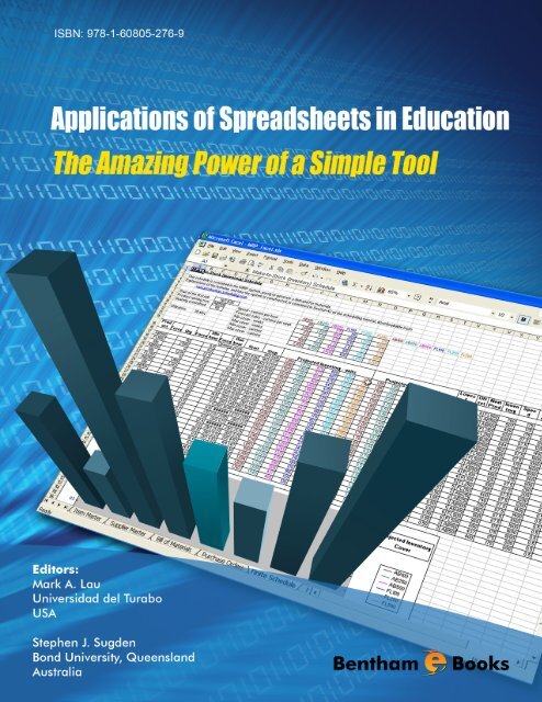
Applications of Spreadsheets in Education 

The Amazing Power of a Simple Tool 

Edited by 

Mark Lau and Stephen Sugden

eBooks End User License Agreement 

Please read this license agreement carefully before using this eBook. Your use of this eBook/chapter constitutes your agreement 

to the terms and conditions set forth in this License Agreement. Bentham Science Publishers agrees to grant the user of this 

eBook/chapter, a non-exclusive, nontransferable license to download and use this eBook/chapter under the following terms and 

conditions: 

1. This eBook/chapter may be downloaded and used by one user on one computer. The user may make one back-up copy of this 

publication to avoid losing it. The user may not give copies of this publication to others, or make it available for others to copy or 

download. For a multi-user license contact permission@bentham.org 

2. All rights reserved: All content in this publication is copyrighted and Bentham Science Publishers own the copyright. You may 

not copy, reproduce, modify, remove, delete, augment, add to, publish, transmit, sell, resell, create derivative works from, or in 

any way exploit any of this publication’s content, in any form by any means, in whole or in part, without the prior written 

permission from Bentham Science Publishers. 

3. The user may print one or more copies/pages of this eBook/chapter for their personal use. The user may not print pages from 

this eBook/chapter or the entire printed eBook/chapter for general distribution, for promotion, for creating new works, or for 

resale. Specific permission must be obtained from the publisher for such requirements. Requests must be sent to the permissions 

department at E-mail: permission@bentham.org 

4. The unauthorized use or distribution of copyrighted or other proprietary content is illegal and could subject the purchaser to 

substantial money damages. The purchaser will be liable for any damage resulting from misuse of this publication or any 

violation of this License Agreement, including any infringement of copyrights or proprietary rights. 

Warranty Disclaimer: The publisher does not guarantee that the information in this publication is error-free, or warrants that it 

will meet the users’ requirements or that the operation of the publication will be uninterrupted or error-free. This publication is 

provided "as is" without warranty of any kind, either express or implied or statutory, including, without limitation, implied 

warranties of merchantability and fitness for a particular purpose. The entire risk as to the results and performance of this 

publication is assumed by the user. In no event will the publisher be liable for any damages, including, without limitation, 

incidental and consequential damages and damages for lost data or profits arising out of the use or inability to use the publication. 

The entire liability of the publisher shall be limited to the amount actually paid by the user for the eBook or eBook license 

agreement. 

Limitation of Liability: Under no circumstances shall Bentham Science Publishers, its staff, editors and authors, be liable for 

any special or consequential damages that result from the use of, or the inability to use, the materials in this site. 

eBook Product Disclaimer: No responsibility is assumed by Bentham Science Publishers, its staff or members of the editorial 

board for any injury and/or damage to persons or property as a matter of products liability, negligence or otherwise, or from any 

use or operation of any methods, products instruction, advertisements or ideas contained in the publication purchased or read by 

the user(s). Any dispute will be governed exclusively by the laws of the U.A.E. and will be settled exclusively by the competent 

Court at the city of Dubai, U.A.E. 

You (the user) acknowledge that you have read this Agreement, and agree to be bound by its terms and conditions. 

Permission for Use of Material and Reproduction 

Photocopying Information for Users Outside the USA: Bentham Science Publishers Ltd. grants authorization for individuals 

to photocopy copyright material for private research use, on the sole basis that requests for such use are referred directly to the 

requestor's local Reproduction Rights Organization (RRO). The copyright fee is US $25.00 per copy per article exclusive of any 

charge or fee levied. In order to contact your local RRO, please contact the International Federation of Reproduction Rights 

Organisations (IFRRO), Rue du Prince Royal 87, B-I050 Brussels, Belgium; Tel: +32 2 551 08 99; Fax: +32 2 551 08 95; E-mail: 

secretariat@ifrro.org; url: www.ifrro.org This authorization does not extend to any other kind of copying by any means, in any 

form, and for any purpose other than private research use. 

Photocopying Information for Users in the USA: Authorization to photocopy items for internal or personal use, or the internal 

or personal use of specific clients, is granted by Bentham Science Publishers Ltd. for libraries and other users registered with the 

Copyright Clearance Center (CCC) Transactional Reporting Services, provided that the appropriate fee of US $25.00 per copy 

per chapter is paid directly to Copyright Clearance Center, 222 Rosewood Drive, Danvers MA 01923, USA. Refer also to 

www.copyright.com

To my wife Keddy and daughter Helga 

for making my mornings brighter and 

for lifting my spirit in the face of adversity 

Mark Lau 

To my sons, Benn and Stephen, 

and my grandsons Nikolas and Marko 

Stephen Sugden

CONTENTS 

Foreword i 

Preface ii 

Contributors v 

CHAPTERS 

1. Fault Analysis in Power Systems 

Mark A. Lau and Sastry P. Kuruganty 

Part I – Engineering 

2. Use of Spreadsheets for Analyses in Structural Engineering 

Nelson Lam 

3. Optimal Control of Dynamical Systems 

Mark A. Lau and William E. Singhose 

Part II – Mathematics and Sciences 

4. Spreadsheet Conditional Formatting Illuminates Investigations into Modular 

Arithmetic 

5. 

6. 

David Miller and Stephen Sugden 

Computational Problem Solving in Context: 

From Arithmetic Sequences to Polygonal-like Numbers 

Sergei Abramovich 

Enzyme Kinetics for Novice Learners: 

Numerical Simulation in Excel 

Scott A. Sinex and Barbara A. Gage 

3 

18 

41 

64 

84 

107

Part III – Management Sciences 

7. Project Management Spreadsheet Gaming Application 

Wee Leong Lee 

8. Teaching Portfolio Theory in an Equilibrium Setting with the Aid of Spreadsheet 

Tools 

Clarence C.Y. Kwan 

9. Forecasting with Innovation Diffusion Models: An Updated Example from the 

Telecommunications Industry 1994-2009 

John F. Kros and S. Scott Nadler 

10. School Mathematics with Excel 

Jan Benacka 

Part IV – General Education 

11. Graduates’ Use of Technical Software in Financial Services 

Timothy Kyng, Leonie Tickle, and Leigh Wood 

12. Professional Development in Electricity Markets with Spreadsheet Models 

Elliot Tonkes 

Subject Index 274 

116 

140 

159 

173 

241 

261

FOREWORD 

A little over 30 years have passed since the first spreadsheet, VisiCalc, made its appearance as an 

exciting and effective computer tool for accounting and business modeling. In the ensuing years, 

educators have increasingly recognized that the spreadsheet has extraordinary potential for other 

applications as well. Today, not only are spreadsheets, as exemplified by Microsoft Excel, among 

the most widely-used modeling and mathematical tools of the workplace, but they also find abundant 

use in diverse areas of education. In addition to business-related areas, usage flourishes in 

mathematics, the natural and social sciences, engineering, and many other areas. The spreadsheet’s 

natural, approachable tabular format and its operations that are acquired readily make it accessible 

to students. With their formidable graphics features, user tools, and programming capabilities, 

spreadsheets are effective tools for teachers, students, and researchers. 

Yet, even today the value of spreadsheets in education is not always fully recognized. To address 

that situation, this book supplies readers with a substantial variety of educational applications for 

spreadsheets, from fields such as engineering, mathematics, science, and business. The diverse 

applications show two principal ways of using a spreadsheet. First, it is a natural tool for designing 

applications directly from first principles and then experimenting with the resulting model. Second, 

it provides an accessible way to implement models and algorithms that are first derived analytically 

by traditional methods. In either way, a major advantage of the spreadsheet approach is to make 

more topics accessible to students that may otherwise be too advanced for them. 

Using the book’s applications, instructors and students can investigate and interrogate the various 

models in the traditional “What if ...?” spreadsheet manner by varying its parameters values. 

They also can visualize the results in both the attractive graphs and the well-designed spreadsheet 

displays that are presented. 

The examples provided include a number that are of a sophisticated nature, showing how 

spreadsheet usage can be extended to more complex problems. Several examples examine models 

that use a difference equation approach that is natural for the spreadsheet medium to implement 

numerical analysis algorithms for topics coming from calculus, linear algebra, and ordinary and 

partial differential equations. 

Throughout the book readers also will encounter the use of powerful tools provided on a spreadsheet 

such as Excel, including built-in and user-designed functions, matrix operations, a solver, 

sliders, and VBA programming. Finally, in addition to providing a wealth of useful examples, each 

chapter contains numerous references and a list of other related topics and problems to pursue, as 

well as ways in which spreadsheet usage can be incorporated into the classroom, assignments, and 

group projects. This book represents a very useful contribution to the literature on the educational 

uses of spreadsheets. 

Deane Arganbright 

Martin, Tennessee, USA 

and Divine Word University, Papua New Guinea 

i

ii 

PREFACE 

This e-book is devoted to the use of spreadsheets in the service of education in a broad spectrum 

of disciplines: science, mathematics, engineering, business, and general education. The effort is 

aimed at collecting the works of prominent researchers and educators that make use of spreadsheets 

as a means to communicate concepts with high educational value. 

Spreadsheets have been around since the late 70s. They were initially conceived as office 

productivity tools, most notably in accounting applications. Over time, spreadsheets evolved to incorporate 

a wealth of functions to appeal to the scientific community. Applications of spreadsheets 

in different branches of science and engineering are continually being reported in many scholarly 

journals. 

In recent years, a shift in learning paradigms towards a more constructivist education has incited 

researchers and educators to find new approaches to education in science, mathematics, and 

engineering. This trend is not confined to the USA only, but it seems that it is more widespread 

around the globe. It is in this context, that applications of spreadsheets in education, from primary 

to university levels, are gaining marked prominence, as evidenced by the number of journal 

publications and presentations at technical conferences. 

This e-book brings some of the most recent applications of spreadsheets in education and research 

to the fore. We assume that the reader is already familiar with the basics of electronic 

spreadsheets. To offer the reader a broad overview of the diversity of applications, carefully chosen 

examples from different areas have been included. Applications have been organized in four parts, 

each containing three chapters: 

• Part I: Engineering 

Chapter 1 presents fault analysis in power systems, a common topic in power system courses. 

Symmetrical and unsymmetrical short circuit currents are computed using a spreadsheet. The 

determination of these currents provides valuable information for selecting the appropriate 

protection equipment in a power system. 

Chapter 2 shows how to implement spreadsheets for structural analysis. The topic is relevant 

to many branches of engineering, namely, civil, mechanical, aerospace, and structural 

engineering. Spreadsheet models for analyzing beams, walls, frames, and multi-degree-offreedom 

systems are presented. 

Chapter 3 discusses optimal control of dynamical systems. The minimum principle of Pontryagin 

and the numerical solution of differential equations are illustrated with spreadsheets. 

In addition, an interesting example motivated by research (control of a flexible structure via 

command shaping) is presented in this chapter.

• Part II: Mathematics and Sciences 

Chapter 4 illustrates modular arithmetic, a topic that is relevant to mathematicians and computer 

scientists. This chapter makes use of the conditional formatting of spreadsheets to 

reveal interesting patterns in modular arithmetic. 

Chapter 5 presents computational problem solving in context. In this chapter, some amusing 

problems involving difference equations, number sequences, and polygon-like numbers are 

solved with the help of spreadsheets. 

Chapter 6 introduces enzyme kinetics to chemistry, biology, and biochemistry students. This 

chapter includes the kinetics of enzyme reactions, linear and non-linear regression analyses, 

experimental error, and the effects of inhibitors. 

• Part III: Management Sciences 

Chapter 7 describes a project management gaming application. The project management 

game is designed as a teaching tool to allow players to experience project management in an 

interactive and fun atmosphere. The game exposes players to project planning, budgeting, 

resource allocation, decision making, and many other aspects of IT projects in a very realistic 

manner. 

Chapter 8 introduces mean-variance portfolio theory, which is part of the core curriculum 

of modern finance in business education. In particular, this chapter presents an asset pricing 

model in an equilibrium setting. Several spreadsheet features in matrix operations are used 

to illustrate the computational task involved. 

Chapter 9 presents a research study on the innovation diffusion model and the life cycle of a 

high technology product applied to the sales of modems from 1994–2009, including successive 

generations of modems: 14.4k, 28.8k, 56k, broadband less than 3.6Mbps, and broadband 

greater than 3.6Mbps. The model is used by managers to understand the development of new 

products and their life cycle. 

• Part IV: General Education 

Chapter 10 exploits the graphical capabilities of spreadsheets to enhance the teaching and 

learning of school mathematics. Topics presented in this chapter include introductory calculus, 

functions, linear algebra, conics, and stereometry. 

Chapter 11 reports a research study on the use of technical software, including spreadsheets, 

by graduates of actuarial studies programs in Australia. The chapter suggests some implications 

for universities wishing to design curriculum to prepare students for careers in the 

financial services industry. 

Chapter 12 presents a case study illustrating the physical dispatch algorithm used by Australia’s 

electricity market operator (AEMO) to determine which power plants to dispatch into 

the grid and the resultant electricity spot price. The spreadsheet model presented in this 

chapter is used in professional development workshops. 

Some of these applications make use of Visual Basic for Applications (VBA), a versatile computer 

language that further expands the functionality of spreadsheets. 

iii

iv 

The chapters contained herein were contributed by prominent researchers and educators who 

made creative use of spreadsheets as a research, teaching, and/or learning tool. The reader can 

download the spreadsheet models presented in this e-book from the publisher’s website. The 

breadth of applications will provide the reader with a fresh look at the amazing power and the 

simplicity of spreadsheets and the VBA programming environment. We hope that the material included 

in this e-book will inspire readers to devise their own applications and enhance their teaching 

and/or learning experience, and share our passion for spreadsheets. 

Acknowledgements 

First and foremost, we wish to acknowledge our great debt to our contributors for sharing their 

expertise. We are grateful to the following people for their valuable comments and diligence in 

reviewing this e-book: John Baker (Natural Maths, Australia), Oscar Chavez (Mathematics Education 

Program, University of Missouri, USA), Greg Cranitch (School of Information Technology, 

Bond University, Australia), Marjorie Darrah (Department of Mathematics, West Virginia University, 

USA), Neville de Mestre (Emeritus Professor, School of Information Technology, Bond University, 

Australia), Therese Donovan (Vermont Cooperative Fish and Wildlife Research Unit, University 

of Vermont, USA), Adrian Gepp (School of Business, Bond University, Australia), Kieran 

Lim (School of Biological and Chemical Sciences, Deakin University, Australia), Thomas Overbye 

(Department of Electrical and Computer Engineering, University of Illinois at Urbana-Champaign, 

USA), Malcolm Peck (Managing Director, The Carnot Group, Australia), Warren Richards (Head 

of Department of Mathematics, Moreton Bay College, Australia), Vladimir Romanenko (North 

Western Institute of Printing, St. Petersburg State University of Technology and Design, Russia), 

Geoff Smith (Department of Mathematics, University of Technology, Sydney, Australia), Michael 

Steele (Faculty of Business, Division of Economics and Statistics, Bond University, Australia), and 

to the anonymous peer reviewers appointed by Bentham Science Publishers. We also want to thank 

Salma Sarfaraz and Hina Wahaj of Bentham for their assistance in making this project a success. 

Mark Lau 

Universidad del Turabo, Puerto Rico, USA 

mlau@suagm.edu 

Stephen Sugden 

Bond University, Queensland, Australia 

ssugden@bond.edu.au 

August 2011

CONTRIBUTORS 


Department of Curriculum and Instruction 

State University of New York at Potsdam, Potsdam, New York, USA 

Jan Benacka 

Faculty of Natural Sciences 

Constantine the Philosopher University, Nitra, Slovakia 

Barbara A. Gage 

Department of Physical Sciences and Engineerin 

Prince George’s Community College, Largo, Maryland, USA 

John F. Kros 

Department of Marketing and Supply Management 

East Carolina University, Greenville, North Carolina, USA 

Sastry P. Kuruganty 

Department of Electrical and Computer Engineering 

Universidad del Turabo, Gurabo, Puerto Rico, USA 

Clarence C.Y. Kwan 

DeGroote School of Business 

McMaster University, Hamilton, Ontario, Canada 

Timothy Kyng 

Department of Actuarial Studies 

Macquarie University, New South Wales, Australia 

Nelson Lam 

Department of Civil and Environmental Engineering 

University of Melbourne, Victoria, Australia 

Mark A. Lau 



v

vi 

Wee Leong Lee 

School of Information Systems 

Singapore Management University, Singapore 

David Miller 

Department of Mathematics 

West Virginia University, Morgantown, West Virginia, USA 

S. Scott Nadler 

College of Business 

University of Central Arkansas, Conway, Arkansas, USA 

Scott A. Sinex 

Department of Physical Sciences and Engineering 


William E. Singhose 

The George W. Woodruff School of Mechanical Engineering 

Georgia Institute of Technology, Atlanta, Georgia, USA 

Stephen J. Sugden 

Faculty of Business 


Leonie Tickle 

Department of Actuarial Studies 


Elliot Tonkes 

Director of Risk and Analytics 

Energy Edge Pty Ltd, Brisbane, Australia 

Leigh Wood 

Faculty of Business and Economics 

Macquarie University, New South Wales, Australia

Part I 

Engineering

Applications of Spreadsheets in Education The Amazing Power of a Simple Tool, 2011, 3–17 3 

Fault Analysis in Power Systems 

Mark A. Lau ∗ and Sastry P. Kuruganty 



CHAPTER 1 

∗ Address correspondence to: Dr. Mark A. Lau, Department of Electrical and Computer Engineering, Universidad 

del Turabo, Road 189 Km 3.3, Gurabo, Puerto Rico 00778-3030, USA; Tel: (+1) 787-743-7979, 

Ext. 4174; E-mail: mlau@suagm.edu 

Abstract: Fault analysis is an important consideration in power system planning, 

protection equipment selection, and overall system reliability assessment. At the 

heart of today’s power generation and distribution are high-voltage transmission and 

distribution networks. When a fault (e.g., a short circuit) occurs at some point in the 

network, the normal operating conditions of the system are upset; if the fault is persistent 

severe loss of load, property damage due to fire or explosion, and steep economic 

losses can arise as undesirable consequences. Therefore, the correct modeling 

of components and the correct fault analysis in power systems are critical to ensuring 

safety and reliability. In this chapter fault analysis is illustrated via spreadsheets. 

Spreadsheets are widely accessible and the ease of programming is the hallmark 

feature that renders them appealing to many users. This simple tool is employed to 

analyze both symmetrical and unsymmetrical faults in power systems. The determination 

of fault currents aids the power engineer in the selection and coordination of 

protective equipment to ensure the safe and reliable operation of the system. 

Keywords: fault analysis, symmetrical faults, unsymmetrical faults, short circuits, power systems. 

1.1 Introduction 

The complexity of power systems demands a variety of tools for their correct modeling, analysis, 

and design. Classical problems such as power (load) flows, transient stability, dynamic stability, 

fault analysis, and economical dispatch are part of the knowledge repertoire of any practicing power 

engineer. 

This chapter discusses fault analysis in power systems utilizing spreadsheets. Fault analysis is 

an important aspect in power system planning, protection equipment selection, and overall system 

reliability. A fault is defined to be an event or condition that disrupts the normal operation of a power 

system. To be more specific, this chapter focuses on short circuits in three-phase power systems. 

Short circuits may be classified under two categories: symmetrical faults and unsymmetrical faults. 

Mark Lau and Stephen Sugden (Eds) 

All rights reserved – c○2011 Bentham Science Publishers Ltd.

4 Applications of Spreadsheets in Education The Amazing Power of a Simple Tool Lau and Kuruganty 

A three-phase short circuit constitutes a symmetrical fault; single line-to-ground, line-to-line, and 

double line-to-ground short circuits are instances of unsymmetrical faults. 

In decreasing order of frequency short circuits in three-phase power systems occur as follows: 

single line-to-ground, line-to-line, double line-to-ground, and balanced three-phase faults. While 

balanced three-phase faults are the least frequent, these faults will be presented first because of their 

conceptual simplicity. The material presented in this chapter is accessible to most undergraduatelevel 

students with some previous exposure to power system concepts. The presentation follows 

those of most textbooks [1–4]; equations are given without derivations as they can be found in 

standard reference books [1–4]. Instead, the emphasis is placed on the construction of spreadsheet 

models to analyze faults in power systems. Applications of spreadsheets in power system analysis 

have been reported in the literature [5–8]. It is along this line that this chapter is presented, 

continuing the efforts initiated by the authors in a power systems course [6, 7]. 

This chapter is organized as follows. Section 1.2 presents a spreadsheet implementation to 

analyze balanced three-phase short circuits. Spreadsheet models for analyzing unbalanced threephase 

faults are presented in Section 1.3. Subsequently, a discussion on the spreadsheet models and 

possible adaptations is given in Section 1.4. Finally, Section 1.6 gives some concluding remarks. It 

is pointed out that throughout this chapter, spreadsheet models are implemented in Microsoft Excel. 

1.2 Symmetrical Faults 

A power system is normally treated as a balanced (symmetrical) three-phase network. When a fault 

occurs, the symmetry is oftentimes upset, resulting in unbalanced phase currents and phase voltages. 

A three-phase symmetrical fault is a special case because it involves all three phases equally at the 

fault location. Fault analysis is typically performed by examining the so called sequence networks 

of the system being analyzed. In fact, any system can be represented by three sequence networks: 

zero-, positive-, and negative-sequence networks. In the special case of a balanced three-phase short 

circuit, the resulting fault currents are balanced and, hence, only the positive-sequence network is 

considered. For more background information on symmetrical components and sequence networks, 

the reader may consult any of the standard books [1–4]. 

It turns out that fault currents resulting from symmetrical three-phase short circuits can be calculated 

from the one-line (or per-phase equivalent) diagram of the system and the pre-fault operating 

conditions. During the fault the phase current and phase voltage undergo a subtransient period, followed 

by a transient period, before settling down to a steady state. To simplify matters and to make 

the analysis amenable to spreadsheet implementation, the following assumptions are made [1–4]: 

1. All system voltages are replaced by a single driving voltage at the fault location. This driving 

voltage is the pre-fault voltage at the fault location. Further, this pre-fault voltage is assumed 

to be the open-circuit voltage at that point. 

2. In most applications, load currents are small in comparison to fault currents and may be 

neglected. 

3. Transformers are represented by their leakage reactances. Winding resistances and shunt 

admittances are neglected.

Fault Analysis in Power Systems Applications of Spreadsheets in Education The Amazing Power of a Simple Tool 5 

4. Transmission lines are represented by their equivalent series reactances. Series resistances 

and shunt admittances are ignored. 

5. Synchronous machines are represented by constant-voltage sources behind subtransient reactances. 

Armature resistance, pole saliency, and saturation effects are ignored. 

To illustrate the analysis of symmetrical faults, consider the five-bus power system whose oneline 

diagram is shown in Fig. (1.1). Machine, transformer, and line data are given in Table 1.1. The 

data are given in per unit (p.u.) of a common base. 

Eg1 

Generator 1 Transformer 1 

jX" d 1 

jXT1 j 0.04 j 0.025 

1 

jX25 

j 0.1 

jX45 

j 0.05 

5 4 

2 

Transmission lines 

j 0.125 

jX24 

Transformer 2 Generator 2 

jXT2 jX" d 2 

j 0.02 

Fig. (1.1): One-line diagram of power system for symmetrical fault analysis. 

Table 1.1: Synchronous machine, transformer, and transmission line data 

Generator 

Bus Subtransient reactance, X ′′ 

d (p.u.) 

1 0.04 

3 0.02 

Transformer 

Bus-to-Bus Leakage reactance, XT (p.u.) 

1–5 0.025 

3–4 0.02 

Line 

Bus-to-Bus Series reactance, XL (p.u.) 

2–4 0.125 

2–5 0.1 

4–5 0.05 

It is also assumed that the pre-fault voltage at the faulted bus is VF = 1.05e j0o p.u. Since 

machine subtransient reactances are used in the analysis, the currents to be calculated are then 

subtransient fault currents. The purpose of the analysis is to determine the subtransient fault currents 

and phase voltages in each bus when a three-phase short circuit occurs at bus 1. The calculations 

are then repeated for three-phase short circuits occurring at bus 2, 3, and so on. 

3 

j 0.02 

Eg2

18 Applications of Spreadsheets in Education The Amazing Power of a Simple Tool, 2011, 18–40 

Use of Spreadsheets for Analyses in Structural Engineering 

Nelson Lam 

Department of Civil and Environmental Engineering 

University of Melbourne, Parkville, Victoria, Australia 

CHAPTER 2 

Address correspondence to: Dr. Nelson Lam, Department of Civil and Environmental Engineering, School 

of Engineering, University of Melbourne, Parkville 3010, Australia; Tel: (+61) 3-8344-7554; E-mail: 

ntkl@unimelb.edu.au 

Abstract: Structural engineering is a branch of engineering that is concerned with 

the analysis and design of elements such as beams, frames, trusses, and other mechanical 

structures whose principal function is to provide the necessary supporting 

feature to withstand the mechanical loads, or related operating conditions, normally 

associated with structures such as buildings, bridges, cranes, airplanes, and so on. 

This chapter concentrates on the analysis of beams, wall frames, and buildings. 

More specifically, the analyses of these structures are illustrated via Microsoft Excel 

spreadsheets. Spreadsheets may be used to develop quite sophisticated applications 

that can automate the intensive calculations commonly encountered in structural 

analysis. 

Keywords: structural analysis, beams, walls, frames, modal analysis. 


Excel spreadsheets are widely used in design offices for providing assistances to the design of 

engineered structures. This type of spreadsheet program is typically used for accessing a database 

of design parameters (for the selection of products, for example) or to expedite the checking of the 

design against a list of criteria for ensuring code compliances. Essentially, Excel spreadsheets have 

been used as database managers to replace the tedious tasks of looking up design charts and tables 

manually, and for checking compliances. 

This chapter is also concerned with the application of Excel in structural engineering design and 

analysis, with an emphasis on the potential usage of the platform for educational purposes and for 

the more intensive analytical tasks that are traditionally performed by proprietary structural analysis 

packages. Such potential uses of Excel that are being explored in this chapter have not been widely 

recognized. 



Use of Spreadsheets for Analyses Applications of Spreadsheets in Education The Amazing Power of a Simple Tool 19 

The use of Excel in educating engineers with elementary structural mechanics is first illustrated. 

The conventional approach to the solution of problems in engineering statics (i.e., calculation of 

shear forces and bending moments) would always require solving simultaneous equations for determining 

the values of the support reactions. It is demonstrated herein that with the use of Excel 

the solution could be obtained very differently by an intuitive approach. For example, the value of 

a vertical support reaction of a simply supported beam can be determined by trial-and-error until 

equilibrium is satisfied (i.e., end-moments at free ends approaching zero values). Embodied in this 

trial-and-error process is the educational objective of having the student visualize the conditions 

of equilibrium through graphical display of the forces and moments surrounding the beam while 

different reaction values are being keyed in. Essentially, the focus of attention is on the physical 

conditions of the beam as displayed graphically, which is in contrast to the conventional treatment 

of the problem by linear algebra. This alternative approach to engineering statics is particularly 

useful to students who are introduced to the concepts for the first time. The teaching of the conventional 

solution method could be introduced subsequently when the underlying concepts have been 

well understood. 

The conventional method of finding deflections of a beam would require finding the values 

of constants in polynomial expressions based on pre-defined boundary conditions. When Excel 

is employed, the solution can be obtained intuitively in two steps: (i) deforming the beam with a 

constant or variable curvature along its length and (ii) rotating the beam (as a rigid body) in the 

vertical plane about a support until the beam is leveled with all the supports. The trial-and-error 

procedure of deforming and rotating the beam about one of its supports serves to engage the students 

into finding the deflection profile by intuition while alleviating the need to become heavily involved 

with algebra. The educational attribute can be further enhanced by the use of interactive graphics 

display in Excel. A similar intuitive approach could be employed for determining the value of the 

reaction at a redundant (say interior) support through visualizing the beam gradually leveling with 

the support point as the reaction value is gradually varied. A full description of the programming is 

presented in Section 2.2. 

Section 2.3 explores the use of standard matrix operations (involving addition, multiplication, 

and inversion of matrices and vectors) for analyzing lateral resisting elements including building 

frames, structural walls, or wall-frame elements. The flexibility matrix of a lateral resisting element 

can be constructed readily once the deflection of the element at every floor level in the building 

has been identified. The flexibility matrix can be inverted in Excel to give the stiffness matrix. 

Importantly, stiffness matrices representing contributions by individual lateral resisting elements 

can be summed to represent joint actions that are facilitated by diaphragm actions of the building 

floors. 

Section 2.4 illustrates the use of Excel for undertaking the more advanced (dynamic) analysis 

of single-story and multi-story buildings. The simulation of the response displacement time-history 

of a single-degree-of-freedom (SDOF) system can be accomplished by what is known as the central 

difference method of step-by-step time integration as is illustrated in Section 2.4.1. The forward 

marching algorithm featured in this solution method can be implemented easily by a column array 

in Excel. Such a column array can be constructed from top to bottom using the fill down command. 

Interestingly, the use of a column array for finding the solution for a SDOF system can be expanded 

into a rectangular array for solving multiple systems, the results of which can be used for plotting 

the response spectra of the applied excitations. The rectangular array can be constructed from

20 Applications of Spreadsheets in Education The Amazing Power of a Simple Tool Nelson Lam 

left to right using the fill right command. The solution of eigenvalues (modal natural periods) 

and eigenvectors (mode shapes) in a dynamic modal analysis could also be calculated by Excel 

as illustrated in Section 2.4.2. The spreadsheet solution features iterations through populating the 

worksheet with column arrays from left to right (using the fill right command). Every iteration 

commences at the column array on the left and then ends at the column array on the right. In 

perspective, the forward marching algorithm, the calculation and plotting of the response spectra 

and the solution of the modal periods and mode shape vectors have all been accomplished by fully 

exploiting the standard row and column operations in Excel. Further details of programming in 

Excel for structural dynamic analysis is given in Section 2.4. Much fuller details of algorithm 

development for structural dynamic analysis and simulations are presented in [1, 2]. The use of 

Excel for analysis of cracked reinforced concrete cross-sections based on the fiber-element approach 

is presented in [3]. Results obtained from the latter program for analysis of cracked reinforced 

concrete can be compared with recommendations in [4, 5]. 

Another important attribute of Excel suitable for engineering education and training is its transparency. 

Conventional programming languages such as Fortran, C++, or Visual Basic present the 

program algorithm in the usual text format, effectively delivering information in one dimension. 

Elaborate algorithms of large computer programs are therefore difficult to follow. In contrast, an 

algorithm in Excel is the worksheet itself, thereby delivering information in two dimensions. Algorithms 

in Excel can be introduced by a sequence of worksheets, each of which presents a snapshot 

of the progressive development of a spreadsheet program (from a blank sheet into its final form). 

The presentation of a worksheet for illustration to the user can be enhanced in a number of ways 

including the use of annotations, the coloring of cells (to identify which are the ones for the input 

of data). Thus, a program in Excel can be introduced to users without the need of a user’s 

manual. Details of every step in the computations are evident in the spreadsheet itself if only row 

and column operations have been used. This enables users to make modifications to the program 

customizing specific needs, while having full knowledge of its operations as well as the underlying 

computations. The blackbox syndrome of a computer program is hence eliminated. 

2.2 Beam Analysis (Elementary Level) 

The teaching of elementary structural mechanics using Excel may begin with the cantilever beam 

for illustration purposes. For any location on the beam which is measured at distance x from its 

free-end, values of 〈x−xi〉 = max(x−xi, 0) are calculated where subscript i denotes the position 

of the applied point force and xi is the distance of the point force Fi measured from the free-end. 

Observe that when x−xi is a positive value, 〈x−xi〉 is taken to be equal to x−xi, or else 〈x−xi〉 

is taken to be equal to zero. This formulation allows the calculation of shear force and bending 

moment values to be generalized into simple one-line expressions as shown by Equations (2.1a) 

and (2.1b) – based on the usual free-body diagram principles and the resolving of forces and taking 

moments about the point of interest. 

SF(x)= 

BM(x)= 

N 

∑ 

i=1 

N 

∑ 

i=1 

Fi〈x−xi〉 0 

Fi〈x−xi〉 1 

(2.1a) 

(2.1b)


Optimal Control of Dynamical Systems 

Mark A. Lau 1,∗ and William E. Singhose 2 

1 Department of Electrical and Computer Engineering 


2 The George W. Woodruff School of Mechanical Engineering 

Georgia Institute of Technology, Atlanta, Georgia, USA 

CHAPTER 3 

∗ Address correspondence to: Dr. Mark A. Lau, Department of Electrical and Computer Engineering, Universidad 

del Turabo, Road 189 Km 3.3, Gurabo, Puerto Rico 00778-3030, USA; Tel: (+1) 787-743-7979, 

Ext. 4174; E-mail: mlau@suagm.edu 

Abstract: Optimal control techniques have numerous applications in engineering, 

economics, finance, biology, medicine, and many other fields. In spite of the utility 

of these techniques, the presentation of the topic of optimal control is normally 

reserved for graduate studies within specialties (e.g., systems engineering). In this 

chapter we present some illustrative examples in optimal control whose numerical 

solutions are obtained using the built-in solver capabilities of spreadsheets. Our 

hope is that the important and interesting topic of optimal control can be introduced 

to undergraduate students in a less intimidating manner when spreadsheets are used. 

Keywords: optimal control, Pontryagin’s minimum principle, dynamical systems. 


Optimal control theory provides the means to drive a machine as fast as possible. Or, it can provide 

a controller that moves a machine in the most efficient possible way. Optimal control can even 

provide the best method for balancing the needs for fast and efficient motion. It is the branch of 

mathematics that furnishes the conditions or techniques for deriving functions (control laws) so as 

to optimize a given criterion (cost functional). The foundations of the theory were established in 

the 1960s thanks to the work of Lev Pontryagin, his collaborators, and Richard Bellman. A typical 

control problem includes: 

1. A cost functional that is a function of state and control variables. 

2. A set of differential equations that models the interactions between control variables and state 

variables. 



42 Applications of Spreadsheets in Education The Amazing Power of a Simple Tool Lau and Singhose 

3. In some optimal control problems, ancillary constraints may be included. For example, fixed 

end states, energy usage, control saturation, and so on. 

The solid mathematical foundations that underpin the theory of optimal control have provided 

the impetus for finding applications in engineering, economics, finance, biology, medicine, among 

other fields. Only a brief outline of the mathematical background will be provided in this chapter; 

for a more detailed study of the subject the reader is referred to some of the classic books in optimal 

control [1–3]. In spite of the elegance of its theory and the richness of applications, most undergraduate 

engineering students receive very limited or no exposure to optimal control. In fact, our 

experience as instructors reveals that the presentation of this topic is normally reserved for graduate 

studies within specialties (e.g., systems engineering) that make use of the theory of optimal control. 

We believe that optimal control theory is filled with profound ideas and that undergraduate engineering 

students will benefit from the study of this topic. It is our intention in this chapter to 

offer an accessible introduction to optimal control with the aid of spreadsheets. In particular, the 

Microsoft Excel Solver tool will be employed to solve optimal control problems. The spreadsheet 

approach has been used in the teaching of undergraduate economics and business courses [4–6]. 

In [4], detailed examples of continuous-time systems with first order dynamics are solved using 

the Solver tool; likewise, [5] uses the same tool to explain the optimization problem in a first 

order, discrete-time system, while [6] presents spreadsheet implementations for solving dynamic 

optimization problems. In this chapter we present some illustrative examples dealing with second 

order, continuous-time systems that might appeal to undergraduate engineering students. 

The reason for using spreadsheets is that most students are familiar with such tools. Additionally, 

spreadsheets are widely available and very straightforward to set up, thus making the programming 

requirement fairly straightforward. The rest of the chapter is organized as follows. Section 3.2 

briefly presents the mathematical background for solving optimal control problems. Subsequently, 

Section 3.3 discusses a number of optimal control examples and solutions using spreadsheets. In 

Section 3.4, we offer our perspective on classroom use, and finally, some concluding remarks are 

given in Section 3.5. 

3.2 Mathematical Background 

3.2.1 Pontryagin’s Minimum Principle 

The most important component of optimal control is the minimization of a cost function, such as 

move time or fuel usage. Here we provide a statement of necessary conditions for the minimization 

of a cost functional. More details can be found in [1–3]. 

Consider a dynamical system modeled by the ordinary differential equation (with ˙ (·) denoting 

the derivative with respect to time) 

˙x(t)=f t,x(t),u(t) 

(3.1) 

together with 

x(t0)=x0, u(t)∈U , t ∈[t0, t f] (3.2) 

where f : [t0,t f]×R n × U ↦→ R n is a continuously differentiable function, x(t) ∈ R n is the state 

vector, and u(t) is an input vector from the set of admissible controls U ⊂ R m . The system is

Optimal Control of Dynamical Systems Applications of Spreadsheets in Education The Amazing Power of a Simple Tool 43 

observed from some initial time t0 to a final time t f . The control u(t) must be chosen so as to 

minimize the cost functional 

J = h t f,x(t f) t f 

+ g 

t0 

t,x(t),u(t) dt (3.3) 

where h : [t0, t f]×R n ↦→R and g : [t0, t f]×R n ×U ↦→R are assumed to be continuously differentiable. 

In order to solve the optimal control problem, Pontryagin created a function that combined the 

system dynamics and the cost function. He called it the Hamiltonian, H , and defined it to be 

H t,x(t),p(t),u(t) = g t,x(t),u(t) + p T (t)f t,x(t),u(t) 

where p(t)∈R n is the costate vector and (·) T denotes vector or matrix transposition. The costate 

vector is obtained from the partial derivatives of the Hamiltonian, with respect to the state variables, 

namely, 

˙p ∗ (t)=−H T 

∗ ∗ ∗ 

x t,x (t),p (t),u (t) 

where(·) ∗ denotes optimal quantities. 

Pontryagin’s minimum principle states that the optimal state trajectory x ∗ (t) resulting from 

application of the optimal control u ∗ (t) must minimize the Hamiltonian. That is, 

(3.4) 

(3.5) 

u ∗ (t)= arg min 

u(t)∈U H t,x ∗ (t),p ∗ (t),u(t) , ∀t ∈[t0, t f], ∀u(t)∈U (3.6) 

If the final state x(t f) is not fixed, then we have the following transversality condition 

p ∗ (t f)=h T x t f,x ∗ (t f) 

where hx is the gradient of h. Equations (3.5)–(3.7) give the necessary conditions for optimal 

control. If x(t f) is fixed, then Equation (3.7) is not needed; in this case p ∗ (t f) = c, for some 

constant vector c. 

3.2.2 The Runge-Kutta Method for Solving Differential Equations 

As stated in the previous section, solving optimal control problems involves solving a system of 

ordinary differential equations. For computer implementation we need a numerical technique to 

obtain solutions. There are many numerical techniques available, but perhaps one of the most 

popular is the Runge-Kutta method [7]. Here we present the Runge-Kutta method in the context of 

the system of differential equations 

 

˙x1(t) = f1 t,x1(t),x2(t), p1(t), p2(t) 

 

˙x2(t) = f2 t,x1(t),x2(t), p1(t), p2(t) 

 

˙p1(t) = f3 t,x1(t),x2(t), p1(t), p2(t) 

 

˙p2(t) = f4 t,x1(t),x2(t), p1(t), p2(t) 

(3.8) 

with given (or assumed) initial conditions x1(0), x2(0), p1(0), and p2(0). 

(3.7)


Spreadsheet Conditional Formatting Illuminates 

Investigations into Modular Arithmetic 

David Miller 1 and Stephen Sugden 2,∗ 

1 Department of Mathematics 

West Virginia University, Morgantown, West Virginia, USA 

2 Faculty of Business 


CHAPTER 4 

∗ Address correspondence to: Dr. Stephen Sugden, Faculty of Business, Bond University, QLD 4229, Aus- 

tralia; Tel: (+61) 7-5595-3325; E-mail: ssugden@bond.edu.au 

Abstract: Modular arithmetic has often been regarded as something of a mathematical 

curiosity, at least by those unfamiliar with its importance to both abstract algebra 

and number theory, and with its numerous applications. However, with the ubiquity 

of fast digital computers, and the need for reliable digital security systems such as 

RSA, this important branch of mathematics is now considered essential knowledge 

for many professionals. Indeed, computer arithmetic itself is, ipso facto, modular. 

This chapter describes how the modern graphical spreadsheet may be used to clearly 

illustrate the basics of modular arithmetic, and to solve certain classes of problems. 

Students may then gain structural insight and the foundations laid for applications to 

such areas as hashing, random number generation, and public-key cryptography. 

Keywords: modular arithmetic, conditional formatting. 


Sometimes described as “clock-arithmetic,” at least at high-school level, modular arithmetic was 

sometimes presented there as bit of a curiosity, with little practical application. Perhaps with the 

advent and dominance of digital timepieces, the “clock-arithmetic” terminology has faded, however 

this field of mathematical study is now more important than ever. Pioneered by Euler, and greatly 

advanced by Gauss in his Disquisitiones Arithmeticae in 1801 [1], modular arithmetic was indeed 

regarded as a curiosity at that time. Given that integer arithmetic on a digital computer is inherently 

modular (see Section 4.2), and that computers permeate our daily lives, it seems somewhat strange 

that our pre-tertiary students learn essentially nothing of the very important topic of modular arithmetic. 

More than this, a working knowledge of modular arithmetic is essential for the mathematical 

study of modern cryptographic systems such as RSA. We believe that the time for this material to 



Spreadsheet Conditional Formatting Applications of Spreadsheets in Education The Amazing Power of a Simple Tool 65 

be included in the school curriculum is long overdue. With just a little effort, this material may be 

made accessible and, hopefully, appealing to secondary school mathematics students. 

In this chapter we show that informative investigations may be carried out using spreadsheets[2] 

and present new spreadsheet-based approaches for computing and illustrating multiplication tables 

for modular arithmetic. The modular arithmetic spreadsheet described in this chapter allows investigation 

of a variety of properties and concepts in modular arithmetic, including that of modular 

inverse, which is essential for understanding of public-key cryptosystems such as RSA. 

4.2 Modular Arithmetic 

Due in significant part to its widespread application to cryptography and coding theory, basic knowledge 

of this important branch of mathematics is now considered almost essential for IT professionals, 

and others. However, in the experience of the authors, relatively few IT graduates seem to 

appreciate that integer arithmetic on a digital computer is none other than modular arithmetic. This 

is so, as all integer operations are performed modulo some power of 2 – it is the nature of a digital, 

binary CPU. All integer arithmetic done on a digital computer is with respect to a maximum word 

size, and therefore is modulo some positive integer. For example, on a contemporary desktop machine, 

an integer may be represented by 32 bits. This means that additions and multiplications will 

be modulo 2 32 (for cardinals), or 2 31 (for signed integers). When two integers are added on such 

a machine, and the sum exceeds the maximum value representable with 32 bits, e.g., 2 32 − 1 for a 

cardinal, then the processor overflow flag will be set, and the sum will only be correct modulo 2 32 . 

In many instances, this situation corresponds to a serious run-time error. However, if we are doing 

arithmetic modulo 2 32 , then we may legitimately ignore the overflow flag, as this is just the result 

we want. 

4.2.1 Rules of the Game 

What is modular arithmetic and how does it work? What are the basic rules? For the most part, 

these are very simple. The first concept we need is that of remainder or residue. Suppose we wish to 

divide 38 by 9. We have 38=(4×9)+2. In this equation, 38 is the dividend, 9 is the divisor, 4 is the 

quotient, and 2 called the remainder or residue. The word residue means “something left over”. By 

definition, it is non-negative and less than the divisor, so it could be zero. In other words, residues 

run from 0 up to one less than the divisor. In some contexts the divisor is called the modulus (plural 

moduli), and we consider this very soon. Given any dividend and a non-zero divisor, the quotient 

and remainder are unique. This is guaranteed by the so-called division algorithm. 

Theorem 4.1 (The division algorithm) Given integers n and d = 0, there exist unique integers q 

(quotient) and r (residue or remainder) such that n=qd+ r and 0≤r≤d− 1. 

Definition 4.1 In Theorem 4.1, the residue r is also written as n mod d. 

Example 4.1 We have 38=(4×9)+2, so 38 mod 9=2. 

Example 4.2 We have−38=(−5×9)+7, so−38 mod 9=7.

66 Applications of Spreadsheets in Education The Amazing Power of a Simple Tool Miller and Sugden 

Remark 4.1 When computing a mod b for specific integers a and b, we may think of adding or 

subtracting as many copies of b from a as required until we finally arrive at a number in the correct 

range, i.e., between 0 and b−1 inclusive. For example, to compute 89 mod 12, keep removing 

(subtracting) twelves until you are left with 5. This can be regarded as removing seven copies of 12, 

or equivalently, dividing 89 by 12 to obtain a quotient of 7 (irrelevant for modular arithmetic) and 

remainder 5 (the important part). Thus, 89 mod 12=5. To compute(−46) mod 12, do pretty much 

the same thing, except that we need to keep adding twelves until we are “in range,” i.e., between 

0 and 11 inclusive. Adding four twelves to (−46) gives us 2, which is the answer. Thus, (−46) 

mod 12=2. 

Exercise 4.1 Verify that the conditions of Theorem 4.1 are satisfied for each of the examples just 

considered. 

4.2.2 Congruence with Respect to a Modulus 

If two integers x and y have the same residue with respect to a given modulus m, i.e., x mod m = 

y mod m, then we say that they are congruent with respect to this modulus and write x≡y(mod m). 

For example, 22 and 40 are congruent with respect to the modulus 6, since they both have remainder 

4 after division by 6. We write 22≡40(mod 6). Another way to think of this is that the numbers 

x and y differ by a multiple of m, i.e., x−y≡0(mod m). Thus, 22≡40(mod 6) as 22 and 40 differ 

by 18, which is a multiple of 6. 

It is important to realize that the congruence x ≡ a(mod m) defines an infinite arithmetic sequence 

of integers. For example, the congruence x≡1(mod 2) defines the sequence of odd numbers: 

... − 7,−5,−3,−1,1,3,5,7, ... This sequence may be written as xn = 1+2n; n∈Z. Notice 

that we transform the congruence x≡1(mod 2) into an equation by introducing a parameter n. 

4.2.3 Arithmetic Operations 

We have seen that a modulus is simply a positive integer to be thought of as a divisor. If we think of 

it this way, then we can imagine that it generates a quotient and a remainder. For modular arithmetic, 

we are interested only in the remainder (residue). Without loss of generality, we deal with positive 

divisors in this chapter. Clearly, zero cannot be a divisor, and we are not interested in m=1 either, 

since remainders are always zero when we divide by 1; thus, m≥2. 

Now suppose a,b,c,d are any integers. We wish to add, subtract, multiply and divide these 

numbers with respect to a particular modulus m≥2. What are the rules? It turns out that, for the 

most part, they are about as simple as we could hope for. For example, suppose a ≡ 2(mod 7) 

and b≡6(mod 7). Then a+b≡(2+6)(mod 7), a−b≡(2−6)(mod 7), a×b≡(2×6)(mod 7). 

More generally, 

If a ≡ c (mod m) and b≡d (mod m) then, for n≥0,we have 

a+b ≡ (c+d)(mod m) 

a−b ≡ (c−d)(mod m) 

ab ≡ cd(mod m) 

a n ≡ c n (mod m)


Computational Problem Solving in Context: 

From Arithmetic Sequences to Polygonal-like Numbers 


Department of Curriculum and Instruction 

State University of New York at Potsdam, Potsdam, New York, USA 

CHAPTER 5 

Address correspondence to: Prof. Sergei Abramovich, Department of Curriculum and Instruction, State 

University of New York, 210 Satterlee Hall, Potsdam, New York 13676, USA; Tel: (+1) 315-267-2541; 

E-mail: abramovs@potsdam.edu 

Abstract: The learning of mathematical concepts can be aided by the use of technology 

and graphical visualization. The use of modern tools can greatly enhance the 

learning experience by encouraging inquiry and deepening one’s understanding. In 

this chapter triangular, square, and polygonal-like numbers are explored in context 

using spreadsheets. The context provides the element of relevance that learners need 

in order to appreciate concepts that might otherwise seem abstract in nature. 

Keywords: contextual problem solving, arithmetic sequences, polygon-like numbers. 


A number sequence in which the difference between any two consecutive terms is a constant is 

called an arithmetic sequence. The simplest example of such a sequence is the sequence of counting 

numbers 1, 2, 3, 4, ..., where the difference between any two consecutive terms is one. Similarly, 

one can consider the sequence of consecutive odd (1, 3, 5, 7, ...) or even (2, 4, 6, 8, ...) numbers 

as arithmetic sequences with the difference two. 

Many problems in mathematics lead to the summation of consecutive counting, odd, or even 

numbers. Finding such sums can be extended to the summation of other arithmetic sequences. 

Partial sums of arithmetic sequences (e.g., 1, 1+2=3, 1+2+3=6, 1+2+3+4=10, and so 

on) form new number sequences known as polygonal numbers [1]. In particular, these numbers, 

having strong connection to geometry, include triangular (1, 3, 6, 10, ...) and square (1, 4, 9, 16, 

...) numbers which can already be found in the elementary school curriculum as links between 

different mathematical concepts (e.g., [2]). 

An arithmetic sequence is one of the most basic concepts of algebra and number theory. The 

study of arithmetic sequences and their partial sums lends itself to the joint use of context and 

technology. In particular, the use of a spreadsheet in teaching algebra and number theory topics 



Computational Problem Solving in Context Applications of Spreadsheets in Education The Amazing Power of a Simple Tool 85 

to students at pre-college level and their future teachers of mathematics has been well documented 

in the literature [3–10]. The current approach to teaching mathematics in context confronts mathematics 

educators with the task of representing traditional number theory concepts in informal way, 

something that gradually develops a path to mathematical ideas through their numerical representation 

in computational environments. Such an approach is suggested below in the form of number 

of “authentic” situations supported by the use of a spreadsheet. 

5.2 Polygonal Numbers and Second Order Difference Equations 

It should be noted that polygonal numbers have a more complicated nature than arithmetic sequences. 

This complexity deals with the fact that whereas the difference between two consecutive 

terms of an arithmetic sequence is a constant, the difference between two consecutive polygonal 

numbers varies as a linear function of their positional rank. Put another way, whereas the first differences 

between two consecutive polygonal numbers form an arithmetic sequence, their second 

differences have constant values. For example, the sequence tn defined recursively 

Δ2tn = tn+2− 2tn+1+tn = 1, t1 = 1, t2 = 3 (5.1) 

represents polygonal numbers of side three, or, alternatively, triangular numbers. The quantity Δ2tn 

in Equation (5.1) is the second difference of the sequence tn. 

Likewise, the sequence sn defined recursively 

Δ2sn = sn+2− 2sn+1+ sn = 2, s1 = 1, s2 = 4 (5.2) 

represents polygonal numbers of side four, known also as square numbers. 

In the last two decades, triangular and square numbers as concepts appropriate for K-12 curriculum 

appeared in a number of mathematics education publications in the United States and elsewhere 

[1, 7, 11–15], including standards for teaching mathematics [2, 16]. This prompts the idea 

of embedding these concepts in a grade-appropriate context enhanced by a spreadsheet as a means 

of motivating mathematical learning. Such a unity of context, mathematics, and technology makes 

it possible to introduce triangular and square numbers as problem-solving tools. 

More generally, the sequence pn defined recursively through its second difference 

Δ2pn = pn+2− 2pn+1+ pn = m−2, p1 = 1, p2 = m (5.3) 

represents polygonal numbers of side m, or, alternatively, m-gonal numbers. Equations (5.1)–(5.3) 

are linear non-homogeneous difference equations of the second order. The description of polygonal 

numbers through a linear difference equation of the second order resembles the definition of 

Fibonacci numbers, the properties of which, however, are quite different from those of polygonal 

numbers. This is due to the fact that Fibonacci numbers are defined by a homogeneous difference 

equation and polygonal numbers are defined through non-homogeneous difference equations. 

One can solve Equation (5.1) as a non-homogeneous difference equation by finding the sum of 

the general solution to the homogeneous equation tn+2− 2tn+1+ tn = 0 in the form t h n = C1+C2n 

and a partial solution t p n = n(n+1)/2. Then tn = t h n +t p n = C1+C2n+n(n+1)/2. Using the initial

86 Applications of Spreadsheets in Education The Amazing Power of a Simple Tool Sergei Abramovich 

conditions introduced in Equation (5.1) it follows that when n=1 one has t1 = 1= C1+C2+ 1 or 

C1 =−C2; when n=2 one has t2 = 3= C1− 2C1+ 3 whence C1 = 0 and C2 = 0. Thus, 

tn = n(n+1) 

, n=1, 2, 3,... (5.4) 

2 

Similarly, Equations (5.2) and (5.3) can be shown to have the solutions 

and 

respectively. 

5.3 Triangular Numbers 

sn = n 2 , n=1, 2, 3,... (5.5) 

pn = (m−2)n2 +(4−m)n 

, n=1, 2, 3,... (5.6) 

2 

5.3.1 Establishing Context for Triangular Numbers 

In what follows, the use of a spreadsheet will be considered, using Pollak’s [17] terminology, in 

a “whimsical” context. While it may be argued that problems of whimsy have only superficial 

connection to the real world [18], the recent use of the term modeling embraces all possible relations 

between mathematics and the world outside it [19]. It appears that one’s perception of what is 

whimsical and what is not largely depends on one’s experience; in fact, many of today’s real-life 

situations seemed like fictions yesterday. Furthermore, the strong relationship that exists between 

modeling and problem solving suggests the importance for the spreadsheet modeling to be carried 

out in a whimsical context that very often provides a powerful cognitive milieu for solving problems. 

For example, Engel [20] explored such “whimsical” contexts as fishing, book reading, and coin 

tossing. It has been shown that each of these contexts is conducive for using modeling strategies as 

means of instruction and developing the habit of seeing possible applications of mathematics. Note 

that context itself does not account for the mathematical content – the latter usually begins with 

a quantitative inquiry into the former, something that may be referred to as mathematization. We 

begin with 

Problematic Situation (PS) 5.1 Once upon a time, Hilton built a hotel in Atlantic City shaped as 

a long parallelepiped with more than 100 rooms on each storey overlooking the waterline of the 

ocean. The 13th storey turned out to be a dangerous place to stay: Every night a ghost visited a 

room there. It was observed (see Fig. (5.1)) that the ghost started with room 1, on the second night 

he emerged in room 3, on the third night he emerged in room 6, then he emerged in room 10, and so 

on. 

After a few such nights the hotel’s manager hired a student from a local college to investigate 

the behavioral pattern of the ghost by using a spreadsheet. More specifically, the manager wanted 

to know:


Enzyme Kinetics for Novice Learners: 

Numerical Simulation in Excel 

Scott A. Sinex ∗ and Barbara A. Gage 

Department of Physical Sciences and Engineering 


CHAPTER 6 

∗ Address correspondence to: Prof. Scott A. Sinex, Department of Physical Sciences and Engineering, 

Prince George’s Community College, Largo, Maryland 20774-2199, USA; Tel: (+1) 301-341-3023; E-mail: 

ssinex@pgcc.edu 

Abstract: Through an interactive Excel spreadsheet and accompanying activity, 

first-year college students explore enzyme kinetics, experimental error, and the behavior 

of inhibitors. Many “what if” questions drive students to discover how a 

variety of parameters influence results. 

Keywords: enzyme kinetics, inhibitors, non-linear regression. 


Enzyme kinetics [1, 2] finds its way into every college biology textbook and usually is mentioned in 

the chemical kinetics chapter of general chemistry textbooks. Because so many biochemical reactions 

[2] are mediated by enzymes, it is important to understand their kinetics. Biology students [3] 

may encounter enzyme kinetics before seeing chemical kinetics in the second semester of general 

chemistry. Enzyme kinetics is a natural extension of chemical kinetics concepts, although, it can appear 

to use a completely different language. Since enzyme kinetics is an important biological topic 

in molecular biology and microbiology, can general chemistry instructors get it into the curriculum? 

This chapter introduces an interactive Microsoft Excel spreadsheet (or Excelet) and accompanying 

guided-inquiry activity to expose students to the kinetics of enzyme reactions, including 

analyzing data, dealing with experimental error, and observing the effects of inhibitors. Data analysis 

by both linear and non-linear regression analyses is covered as well as analysis of experimental 

results. The use of Excelets as discovery learning tools has been recently described in [4, 5]. 

To use this Excelet, students need Microsoft Excel with the Analysis ToolPak and Solver Add-in 

loaded (instructions are included in the Excelet on the needed Add-ins tab). Students will navigate 

using the tabs at the bottom of the screen (see Fig. (6.1)). Students should have an introduction to 

using the interactive features of Excelets and how to explore a variable beforehand. Data analysis is 



108 Applications of Spreadsheets in Education The Amazing Power of a Simple Tool Sinex and Gage 

Fig. (6.1): Tabs on Excelet. 

handled by the “just add data” aspect of the Excelet, where all graphs and calculations are already 

set up. Students need to know the basics of mathematical modeling (e.g., regression, goodness-offit, 

and so on) as described in [6]. 

6.2 The Kinetics of Enzyme Reactions Excelet 

To get the most out of this discussion, the reader needs to open the interactive Excel spreadsheet 

and accompanying activity. First we review some basic information from chemical kinetics and 

link to other Excelets that review the basic concepts even further. Understanding this information 

is required if students are going to grasp enzyme kinetics. 

We are investigating the classic reaction with the rate constants as given by 

S+E 

k1 

−−−−⇀ ↽−−−− 

k2 

ES 

kcat 

−−−−−→ E+ P (6.1) 

where S is the substrate, E is the enzyme, ES is the enzyme-substrate complex, and P is the product. 

The calculations are similar to concepts outlined in [7] and can demonstrate the validity of the steady 

state approximation. The similarity of enzyme kinetics to homogeneous catalysis is shown in [8], 

wherein some elucidating points on the mechanisms occurring in enzyme kinetics are illustrated. 

This Excelet uses manipulatable variables that feed into the Michaelis-Menten equation to calculate 

the initial velocity of the reaction, v0, on the kinetics plot tab according to 

where 

v0 = vmax(S) 

KM+(S) 

vmax = kcat(E)0 and KM = k2+ kcat 

The kinetics plot tab illustrates a variety of enzymes with substrates. We are trying to get 

students to see how these substrate/enzyme variables influence the graph. How vmax and KM are 

determined from the graph is also illustrated. 

Students then explore the behavior of the concentrations of the substrate, enzyme, enzymesubstrate 

complex, and the product over time on the S, E, & P over time tab by changing the various 

rate constants (k1, k2, and kcat) and initial concentrations of substrate, (S)0, and enzyme, (E)0. 

This part of the Excelet is a system’s dynamic model that uses difference equations to calculate 

concentrations over time. The actual mathematical equations (differential equations converted to 

k1 

(6.2) 

(6.3)

Enzyme Kinetics for Novice Learners Applications of Spreadsheets in Education The Amazing Power of a Simple Tool 109 

difference equations or see [7]) are given on this tab of the Excelet if you scroll down below the 

graph, a sample of which is shown in Fig. (6.2). 

Fig. (6.2): Concentration over time plot. 

A similar plot is employed on the Initial Rate S tab that shows how the initial rate, which is a 

common measurement in enzyme experiments, is determined from the graph. 

6.3 Transformed Data 

If the enzyme kinetics data follows the form of the Michaelis-Menten equation then mathematically 

it is a rectangular hyperbola and can be fit by non-linear regression techniques or the data can be 

transformed to a linear plot and fit using linear regression. We look at the common transformations 

(Table 6.1) used by biochemists [9] to fit the data to find the various parameters: vmax, KM, and kcat 

(see transformed data tab). Historically, the data were transformed to produce linear plots, which in 

the pre-technology age was the only way to analyze the data (using rulers and graph paper). Analysis 

improved with the addition of linear regression, especially employing computational technology. 

A big advantage of linear plots is the ability to spot behavior that is non-linear. Many errors that 

occur when using the transformed data are pointed out in [10]. 

The three plots corresponding to the transformations in Table 6.1 are shown in Fig. (6.3) with 

the lowest concentration value as a green point. One might notice how the points are not regularly 

spaced, especially on the Lineweaver-Burk and Eadie-Hofstee plots. We explore these three 

methods simultaneously and their sensitivity to random and systematic error, both constant and 

proportional. If students need an introduction to investigating error, see [11, 12].


Project Management Spreadsheet Gaming Application 

Wee Leong Lee 

School of Information Systems 

Singapore Management University, Singapore 

CHAPTER 7 

Address correspondence to: Dr. Wee Leong Lee, School of Information Systems, Singapore Management 

University, 80 Stamford Road, Singapore 178902; Tel: (+65) 6828-0937; E-mail: wllee@smu.edu.sg 

Abstract: This chapter seeks to illustrate how simple spreadsheets can be used creatively 

with amazing outcomes. This will be demonstrated through a project management 

game, built entirely using standard spreadsheet features and functions. The 

project management game is designed as a teaching tool to allow players to experience 

project management in an interactive and fun atmosphere. In the game, players 

learn to respond to unforeseen events, make appropriate decisions to resolve issues, 

keep the project team motivated, and take corrective measures to keep the project on 

track and on target. This chapter is aimed at providing an overview of the game, discussing 

how it should be played, and explaining the underlying principles behind the 

rules of the game. It is not meant to be technical, although some amount of logical 

relationship between variables and mathematical functions will be discussed. 

Keywords: project management, gaming applications. 


Spreadsheets were originally intended to help ease laborious accounting work but their applications 

have extended far beyond just crunching numbers, accredited to their versatility and ease of use. 

Today they have become one of the most commonly used applications both in school and at work. 

The use of spreadsheets as teaching tools has also gained popularity in recent years. Spreadsheets 

have been extensively applied to numerous fields, ranging from engineering, statistics, operations 

management, business modeling, and Monte-Carlo simulations [1–3]. 

Microsoft Excel has been the predominant spreadsheet application for many years given the 

pervasive Microsoft Windows platform. The built-in VBA (Visual Basic for Applications) programming 

language in Excel has greatly enhanced its application beyond the normal usage of spreadsheets. 

Numerous games have been developed in Excel spreadsheets and are shared freely over the 

internet. In the course of developing a module in IT projects and vendor management, I looked at 

what has been done in this area using spreadsheets. I found numerous templates for project plan- 



Project Management Spreadsheet Applications of Spreadsheets in Education The Amazing Power of a Simple Tool 117 

ning, budgeting, and Gantt charts. These templates although useful and easily adoptable with little 

training did not meet my expectations. I needed a more interactive application that could serve as 

a teaching tool to allow students to relate to project management concepts and best practices. My 

search was quite exhaustive but I was unable to find an application in Excel that suited my purposes. 

However, I did find some commercial websites selling project management simulation tools. 

Having evaluated some of these commercial project simulation tools, which are often complex, not 

user-friendly and costly, I shelved the idea of incorporating them for my course. 

Having taught a course (Computer as an Analysis Tool) which uses spreadsheets as problem 

solving and modeling tools over four years, I gathered I should have sufficient knowledge and skill 

sets to build an Excel-based project management game. I have never looked back. The process of 

building the game although agonizing at times has turned out to be a very fulfilling and enriching 

experience. Excel is an excellent tool for building an application quickly without messing with 

database, user-interfaces, and reporting tools. All these functionalities can be developed relatively 

easily in Excel albeit scalability could be an issue in the long run. The ease of creating user interfaces, 

rich library of mathematical functions, ease of storing and retrieving data (without having 

to handle large arrays), and simplicity of the coding in VBA programming language reduce the 

development effort considerably. 

A simulator is not to be confused with simulation. A simulator requires the user to respond 

interactively to requests and events in real-time and their responses to those requests and events 

will have consequences (e.g., a flight simulator). A simulation, on the other hand, usually requires 

the user to set up the initial simulation parameters before running the simulation. The outcomes 

can only be known after the simulation is completed and no action is needed while the simulation 

is running. The project management game I developed requires the player to set up a project plan 

(i.e., initial simulation parameters) before executing the plan (i.e., responding to changes). Project 

managers have to manage multiple performance indexes and make critical decisions to situations 

that often result in tradeoffs between the performance indexes. Unforeseen events beyond the control 

of project managers can occur that require good judgment and decision making in order to steer 

the project toward successful completion. 

The project management life cycle can be broadly categorized into three stages, namely, project 

planning, project execution, and control and project closing. Each stage is equally important to ensure 

project success although I chose to only focus on the project planning and project execution 

and control in the game to begin with. In this chapter, I will elaborate more on the planning stage 

while briefly touching on the execution and control stage. The chapter is not meant to be too technical, 

although some amount of logical relationship between variables and mathematical functions 

is discussed. 

7.2 About the Game: Structure and Features 

The project management game is designed as a teaching tool to allow players to experience project 

management in an interactive and dynamic environment. In the game, players learn to respond to 

unforeseen events, make appropriate decisions to resolve issues, keep the project team motivated, 

and take corrective measures to keep the project on track and on target. Throughout the gaming 

exercise, players get to appreciate and experience the complexity of project management in an

118 Applications of Spreadsheets in Education The Amazing Power of a Simple Tool Wee Leong Lee 

intense and yet exciting way, and learn the intricacies of managing project tradeoffs among budget, 

schedule, quality, and motivation. 

In the game players are to plan and manage a virtual IT project. The project consists of a series 

of interdependent activities and players would have to manage the completion of these activities 

while satisfying some performance criterion. There are two parts to this game. Firstly, players 

have to create a project plan by assigning suitable resources to a set of predefined activities. Upon 

completion of the initial project plan, which consists of building the project Gantt chart by assigning 

resources to activities, players shall advance to the second part, executing the project. Events and 

situations will emerge throughout the project execution and players have to exercise good project 

management skills and judgment to steer the project toward completion. 

The game hopes to achieve the following learning outcomes: 

• Understand the importance of effective resource planning in a project. 

• Understand the usage of basic project management tools (e.g., Gantt charts, network diagram, 

resource utilization). 

• Learn to execute a project effectively. 

• Make rational decisions and exercise good judgment under stress and time constraints. 

• Respond appropriately when faced with typical issues in project management. 

• Manage tradeoffs among different performance criteria. 

7.2.1 Game User Interface 

The main user interface (UI) screen of the game is shown in Fig. (7.1). This application was built 

in Excel 2007 utilizing only standard Excel features and functions and VBA without add-ins to 

minimize potential compatibility issues. The main UI consists of dials, indicators, and buttons. On 

the top left corner of the screen is a simulation clock (built using a pie chart) which starts operating 

only when project execution starts. The clock does not run during the project planning stage. A 

complete cycle of the clock represents one simulation day, which is around three minutes in real 

time. An indicator below the clock displays the current day. The first day of the project execution 

is set to January 1st, 2009. 

The decision score (DS) on the right of the UI shows the percentage of decisions made that 

were correct. The customer satisfaction index (CSI) shows the customer level of satisfaction on the 

project performance. The CSI is computed as a function of the performance index as well as the 

overall management of the project. 

The purple and orange buttons on the left of the UI leads to information about activities, employees, 

resource allocation, resource training, network diagram, resource Gantt chart, and schedule 

Gantt chart. The two green buttons are for making decisions and reading emails when prompted by 

the game controller (the game engine that controls the logic). The three light blue buttons off the 

center of the UI toward the right are for making adjustments to the project scope, setting quality 

review dates, and scheduling of meetings, and organizing activities. The four dark blue buttons 

are used for viewing historical performances of the four performance indexes during the game. The

140 Applications of Spreadsheets in Education The Amazing Power of a Simple Tool, 2011, 140-158 

Teaching Portfolio Theory in an Equilibrium Setting 

with the Aid of Spreadsheet Tools 

Clarence C.Y. Kwan* 

DeGroote School of Business 

McMaster University, Hamilton, Ontario, Canada 

CHAPTER 8 

*Address correspondence to: Prof. Clarence C.Y. Kwan, DeGroote School of Business, McMaster University, 

1280 Main Street West, Hamilton, Ontario L8S 4M4, Canada; Tel: (+1) 905-525-9140, Ext. 23979; E-mail: 

kwanc@mcmaster.ca 

Abstract: Mean-variance portfolio theory being part of the core curriculum of modern 

finance in business education, this chapter presents an asset pricing model based 

on it in an equilibrium setting. Here, equilibrium pertains to matching of supply and 

demand of individual assets in an investment market for rational portfolio decisions. 

An example utilizing various Microsoft Excel features in matrix operations is provided 

to illustrate the computational task involved. This chapter is intended to make 

the model less abstract, thus complementing the textbook materials on the model. 

With computational issues no longer a concern, students can focus their attention on 

the concepts involved. 

Keywords: portfolio theory, capital asset pricing model, CAPM. 


Mean-variance portfolio theory is part of the core curriculum of modern finance in business education. 

The theory, which explains those concepts underlying portfolio investment decisions under 

risk – with risk represented by the variance of the probability distribution of rates of returns of the 

investment – has two complementary aspects. As normative theory, it provides criteria for investment 

decisions and stipulates rules for attaining the desired ends. By treating the estimated means, 

variances, and covariances from a multivariate probability distribution of returns on the individual 

financial assets considered as input parameters, it seeks to achieve optimal risk-return tradeoff in the 

allocations of investment capital under various constraints. This task is commonly called normative 

portfolio analysis or, simply, portfolio analysis. As positive theory, in contrast, portfolio theory 

attempts to explain and predict phenomena in investment markets. For example, it allows the collective 

investment decisions by participating investors to determine asset prices or expected returns, 

under the condition of matching supply and demand of financial assets in market equilibrium. 


All rights reserved - © 2011 Bentham Science Publishers Ltd.

Teaching Portfolio Theory Applications of Spreadsheets in Education The Amazing Power of a Simple Tool 141 

Under some simplifying assumptions, such as risk-free lending and borrowing at the same interest 

rate and frictionless short sales of risky assets, the corresponding results of normative portfolio 

analysis are generally easy for students to follow. 1 The assumption of frictionless short sales is that 

the short seller not only provides no cash deposits for any borrowed assets, but also has immediate 

access to the short-sale proceeds for investing in other assets. Once the formulation for constrained 

optimization is in place, the portfolio allocation results will follow. 2 The use of electronic spreadsheet 

tools also helps greatly in reducing the computational burden and in making the analytical 

material involved less abstract to students. As illustrated in [2, 3], with the aid of Microsoft Excel 

features, to construct practically relevant portfolios without using multivariate calculus tools is also 

possible. 3 

The Capital Asset Pricing Model, which is also known simply as the CAPM, is the central 

result of portfolio theory. The model, which is based on the work of [4–6], is highly important in 

modern finance and thus is part of the core curriculum. As mentioned in most introductory finance 

textbooks, the model explains asset pricing in terms of the part of the risk that cannot be diversified 

away from portfolio investments. The Sharpe-Lintner version of the model in [4, 5] establishes, in 

market equilibrium, a tradeoff between the expected return of each asset and its non-diversifiable 

risk. Market equilibrium pertains to matching supply and demand of the individual assets. However, 

the Mossin version in [6] captures explicitly asset prices and the participation of individual investors 

in the model formulation; it allows asset prices instead of their expected returns to be determined. 

The CAPM covered in finance textbooks is the Sharpe-Lintner version. As asset prices are 

implied in the model by their expected returns, a typical question to the author (as an instructor 

of various finance courses in which the CAPM is taught) from students, especially those who are 

unaware of its derivation, is why it is called a pricing model when asset prices are not even there. 

Another typical question from students who have learned normative portfolio analysis is whether 

any expected returns, variances of returns, and covariances of returns are input parameters or results 

of the equilibrium analysis involved. Further, as the market portfolio – which is a portfolio of all 

risky assets in the market providing the best risk-return tradeoff – plays a crucial role in the CAPM, 

some students are also curious as to whether the risk preferences of investors in the market affect 

the risk premium of such a portfolio, in terms of its expected return in excess of the risk-free interest 

rate. These questions can be answered more easily if the derivation of the CAPM is based on an 

analysis where asset prices are explicitly considered. 

Drawing on [7], which is based on a similar idea of the Mossin version of the CAPM, this 

chapter derives an asset pricing model that is less abstract, from a pedagogic perspective. For 

students to understand fully the derivation, they must still have some prior knowledge of various 

economic, mathematical, and statistical topics. The statistical component of the task is generally 

familiar to business students the author has taught, and the idea of equilibrium analysis, though 

likely new to these students, is not complicated. The mathematical component of the task requires 

1 See, for example, Chapter 6 in [1]. 

2 The assumption of frictionless short sales ensures that essential multivariate calculus tools are adequate for the analysis 

involved. If realistic short-sale transactions are to be captured or if short sales are disallowed, then the corresponding 

analysis will be much more complicated. See, for example, [2, 7] for analytical details. 

3 Specifically, [3] uses Excel Solver to construct efficient portfolios, thus bypassing the analytical details of the 

constrained optimization considered. In [2], where the analytical solutions are obtained by using algebraic tools instead, 

the computations involved are performed by using Excel functions for matrix operations.

142 Applications of Spreadsheets in Education The Amazing Power of a Simple Tool Clarence C.Y. Kwan 

the use of multivariate calculus for optimization and matrix algebra. For students who have learned 

normative portfolio analysis, however, such a task is not burdensome. Notice that the equilibrium 

analysis to be presented in this chapter is not intended to replace the textbook version. Rather, the 

two versions complement each other, so that students can better appreciate the various implications 

and limitations of the model. 

The matrix operations as required for the equilibrium analysis here are confined to matrix addition, 

multiplication, transposition, and inversion, as well as finding the determinant of a matrix. As 

spreadsheet tools for matrix operations are easy for students to learn, using them can significantly 

reduce the computational burden. With the relevant input parameters arranged as blocks of data in a 

spreadsheet, to perform matrix operations is straightforward. With computational issues no longer 

a concern, students can focus their attention on conceptual issues pertaining to the model. 

To facilitate the analysis that follows, Section 8.2 first provides some essential material on risk 

aversion. Section 8.3 starts with a basic equilibrium analysis for asset price determination. An 

extension of the analysis, by relaxing a simplifying assumption in the CAPM, is also considered. 

Implications of this extension are discussed as well. Section 8.4 presents an Excel example to 

illustrate the required computations. Section 8.5 offers some concluding remarks. For readers who 

are unfamiliar with the CAPM, the appendix at the end of this chapter provides an abbreviated 

version of its derivation in textbooks. 4 

8.2 Preliminaries 

Let U(W) be the utility function of an investor with wealth W. The investor is rational if the first 

derivative of U(W), written as U ′ (W), is positive. The idea is that, if wealth is the only factor in 

the determination of satisfaction, a rational investor must prefer more wealth to less wealth. The 

investor is also risk averse if the second derivative, U ′′ (W), is negative. The idea is that a risk 

averse investor considers the increase in satisfaction for having an incremental wealth ΔW less than 

the decrease in satisfaction for losing the same ΔW. To illustrate, if an investment has equal chances 

of gaining $h or losing $k, a risk averse investor will not find the investment worthwhile if h≤k; 

exactly how high h−k has to be for the investment to appeal to the investor depends on the function 

U(W). 

For a risk averse investor with an initial wealth W0, suppose that an investment will result 

in W0+z as the final wealth for the investor, with the outcome of the investment z being random. 

To assess the investment, the investor considers the expected utility of all potential outcomes, 

E[U(W0+z)]. Here, E[·] represents the expected value of the variable[·] in question. To the investor, 

this risky investment is equivalent to a risk-free investment with a certain outcome of E[z]−π, 

where π > 0 can be viewed as a premium that the investor is willing to pay in order to avoid risk. 

To determine π, we can start with 

U(W0+ E[z]−π)=E[U(W0+z)] (8.1) 

where W0+ E[z]−π is called the certainty equivalent wealth, CEQ. 

4 See, for example, Chapter 6 in [8].


CHAPTER 9 

Forecasting with Innovation Diffusion Models: An Updated Example 

from the Telecommunications Industry 1994-2009 

John F. Kros 1,∗ and S. Scott Nadler 2 

1 Department of Marketing and Supply Management 

East Carolina University, Greenville, North Carolina, USA 

2 College of Business 

University of Central Arkansas, Conway, Arkansas, USA 

∗ Address correspondence to: Dr. John F. Kros, Department of Marketing and Supply Management, College 

of Business, East Carolina University, 3121 Harold Bate Building, Greenville, North Carolina 27858, USA; 

Tel: (+1) 252-328-6364; E-mail: krosj@ecu.edu 

Abstract: Managers have long been concerned about new product development 

and the life cycle of these products. Because many products do not sell at constant 

levels throughout their lives, product life cycles must be considered when developing 

sales forecasts. Innovation diffusion models have successfully been employed to 

investigate the rate at which goods and/or services pass through the product life 

cycle. This research investigates innovation diffusion models and their relation to 

the product life cycle. The model is developed and then tested using modem sales 

from 1994–2009. Each successive generation of modem innovation, from 14.4k, 

28.8k, 56k, broadband less than 3.6Mbps, to broadband greater than 3.6Mbps, is 

examined. 

Keywords: innovation diffusion model, forecasting, logistic growth model. 


The generation of new product opportunities has been a major area of study in both the academic 

and practitioner literature for decades. Products are born, grow to maturity, and are then either 

reinvented or die. During this ongoing process some products are cast aside by a changing society 

as consumer’s needs and wants change. Business managers are an integral part of this cycle which 

is commonly referred to as the product life cycle (PLC) [1]. 

The PLC is made up of four distinct stages (see Fig. (9.1)). These stages include: introduction, 

growth, maturity, and decline. 



160 Applications of Spreadsheets in Education The Amazing Power of a Simple Tool Kros and Nadler 

Fig. (9.1): Product life cycle. 

During the introduction stage of the PLC the firm’s primary goal is to get the technology into the 

customers’ hands. Growth during the introduction stage of the PLC is generally slow. The second 

or growth stage of the PLC is characterized by its rapid growth as consumers accept the product. 

During the maturity stage of the PLC sales reach the maximum point and the rate of adoption begins 

to fall. In the final stage of the PLC (decline) sales begin to decline significantly as customer needs 

change and they begin adopting newer technologies [1]. 

An important aspect of the PLC is the rate at which consumers adopt a given product or technology. 

There are five categories of adopters. These categories include innovators, early adopters, 

early majority, late majority, and laggards. 

1. Innovators comprise approximately 2.5% of adopters. This group is generally younger and 

more accepting of new technologies. 

2. The second category of adopters is commonly referred to as early adopters. Early adopters 

make up approximately 13.5% and are important because they are known for seeking out new 

technologies. 

3. The third category (early majority) accounts for 34% of the market. The early majority are 

known for being neither the first or last to adopt a new product or technology. Products or 

technologies that have gained acceptance by early majority can no longer be considered new 

as their presence is a known quantity.

Forecasting with Innovation Diffusion Applications of Spreadsheets in Education The Amazing Power of a Simple Tool 161 

4. The fourth or late majority stage makes up another 34% of the market. Late majority adopters 

do not adopt products until after all risks have been identified and when the adoption becomes 

an economic necessity or when there is social pressure to adopt. 

5. The fifth and final stage, which accounts for the final 16% of the market are commonly 

referred to as laggards. Laggards frequently wait to adopt a new technology until the next 

technology generation has entered the market. 

Fig. (9.2) provides a graphic representation of the adopter categories [2]. 

Fig. (9.2): Distribution of adopter categories. 

The constant examination of products as they move through their life cycles is crucial to a firm’s 

success. Managers are challenged with developing new strategies, examining ongoing strategies, 

and eliminating non-competitive strategies for a product’s diffusion into markets. Many times it is 

the primary job of the operations and marketing managers to forecast a product’s diffusion. Within 

the business discipline the product life cycle and forecasting can be linked using what is called 

innovation diffusion theory [3]. 

Innovation diffusion theory has received considerable attention since its inception in the 1960’s. 

The diffusion of innovation can be defined as the process by which an innovation is imparted on 

members of society through certain channels over time [4]. Seminal works in the area of technological 

change and rates of imitation were completed by Fourt [5] and Mansfield [6]. A detailed 

discussion of using diffusion models in product forecasting can be found in [7]. The work by 

Fourt [5] and Mansfield [6] are the basis for research in diffusion modeling by Bass [8]. 

The Bass model for new product growth and innovation diffusion has been used to forecast 

numerous products in many different industries [5, 6, 8–13]. A comprehensive review of the contributions 

to this literature through the 1970’s is provided in [14] and on into the 1980’s in [15]. 

An excellent article comparing nine growth and innovation diffusion models, including Mansfield’s 

and Bass’ models, can be found in [13]. The influence of information technology diffusion on large 

and small businesses is discussed in [9, 10]. Additional insights are provided in [16–20]. 

This chapter extends the work by [21] to the original Mansfield model applied to the technology 

industry where successive generations of the technology exist. The model is developed and then 

tested using modem sales from 1994-2009. The diffusion model is applied to each successive 

generation of modem innovation: 14.4k, 28.8k, 56k, broadband < 3.6Mbps, and broadband > 

3.6Mbps. Two forecasting models for the > 3.6Mbps technology are developed, analyzed, and 

reported on.


School Mathematics with Excel 

Jan Benacka 

Department of Informatics 

Constantine the Philosopher University, Nitra, Slovakia 

CHAPTER 10 

Address correspondence to: Dr. Jan Benacka, Department of Informatics, Faculty of Natural Sciences, 

Constantine the Philosopher University, Tr. A. Hlinku 1, SK-94974 Nitra, Slovakia; Tel: (+421) 37-6408- 

678; E-mail: jbenacka@ukf.sk 

Abstract: The use of computers is pervasive in education at both the secondary and 

university levels. Learner-oriented computer programs have the potential to motivate 

students to learn mathematics. One such computer program is Microsoft Excel, 

which for many years has been embraced by educators as the ideal platform for 

providing students with hands-on activities that enhance their learning. By design, 

Excel (or spreadsheets in general) lends itself to transparent problem formulation 

and minimal programming requirements. 

In this chapter I will present several spreadsheet applications that I have developed 

over the years. The applications are aimed at introducing concepts in the teaching 

of mathematics at the secondary level and introductory calculus as well. 

Keywords: calculus, linear algebra, Euclidean geometry, stereometry. 


During my 14 year teaching practice at grammar school (ages 15–19) where I taught mathematics, 

physics, and informatics in common, mathematical, and informational classes, I started developing 

spreadsheet applications for visualizing mathematical relationships. I have developed the following 

sets of applications: 

• Elementary functions 

• General functions and calculus (derivatives, integrals, and so on) 

• Equations, inequalities without a parameter 

• Equations, inequalities with a parameter 

• Systems of linear equations 



174 Applications of Spreadsheets in Education The Amazing Power of a Simple Tool Jan Benacka 

• Complex numbers 

• Analytical geometry of linear figures in E2 and E3 

• Analytical geometry of quadratic figures in E2 (conic sections, also versus line) 

• Stereometry (sections of cubes, cuboids, prisms, and pyramids; distances and angles of lines 

and planes within these bodies) 

• Functions of two variables 

I have tried the applications at various schools of secondary and university level with very positive 

responses from the students and teachers – some of them were entranced by the possibilities of 

Microsoft Excel and the simplicity of use of the applications. In this chapter I present several 

examples, some of which may be implemented in 5 minutes each provided the student is skilled in 

spreadsheets. In the next sections I will describe eight sets of these from a usage viewpoint. The 

skills required for the applications are: 

(a) writing in the equation of a function, 

(b) fill down, fill right, 

(c) copy formulas into the cells, 

(d) making use of Goal Seek and Solver, 

(e) adjusting axis ranges and units. 

Action (a) cannot be made by a macro. Actions (b) and (c) can be combined together by a macro 

activated by, say, a button. I think I will pursue this approach in my future work. Action (d) can 

be automated by a macro if a value close to the solution is added in a cell; however, I regard Goal 

Seek and Solver so essential in math, useful and easy to use that I will not explore this alternative. 

Action (e) is performed by a macro in various ways in the applications. The axis ranges and units 

are adjusted automatically after inputting the values in cells “xmax”, “xmin”, “ymax”, and “ymin” 

in the charts in Sections 10.2.2 and 10.2.3. Shifting the coordinate system in the left-right or up-left 

direction is possible in Sections 10.4.1 and 10.4.2. Diminishing or enlarging the scene is possible 

in all charts. 

10.2 Functions, Calculus, Equations, Inequalities, and Linear Systems 

10.2.1 Elementary Functions 

Elementary functions are a significant part of mathematics curriculum in school. Students study the 

properties of the graphs, the relations between the parameters and the graph, and so on. The curriculum 

starts with the linear and quadratic functions. Then, there is the linear fractional function, 

integer power function, square root function, exponential and logarithmic function, and trigonometric 

functions.

School Mathematics with Excel Applications of Spreadsheets in Education The Amazing Power of a Simple Tool 175 

To draw the graph of a function by hand, students usually make a table of (x,y) pairs, where 

x goes from about −5 to 5 in increments of 1 and y is calculated according to the equation of the 

function. Then they draw the (x,y) points in xy coordinate system, and draw the graph through the 

points. The accuracy and aesthetic level are minimal. The graphs are static and do not enable students 

to experiment. However, there is a simple tool for making the same more quickly, accurately, 

and at a high aesthetic level – the spreadsheet program. Spreadsheet graphs can easily be made interactive, 

which enables students to experiment with the inputs. Once the application is ready, it can 

be saved and used any time the user needs to study it. In this way, a set of ready-to-use applications 

can be made, one for each elementary function, thus saving valuable time since the user does not 

have to spend effort in creating these applications. The necessary skills can be found in [1, 2]. 

In this chapter, a set of ready-to-use applications for teaching and learning elementary functions 

is presented. I developed them during my 14-year experience in teaching the topic at grammar 

school. There is an application for each elementary function. The models do not require any prior 

knowledge of the applications; the only task is just inputting the parameters, which makes them 

convenient for immediate integration into the teaching process in school as well as learning at home. 

The models enable the user to reveal the meaning of the parameters, find the relations between them 

and the graph, and comprehend it. The possibility of free experimentation due to interactivity and 

simplicity of the models makes them ideal tools for getting the graphs and the meaning of the 

parameters in the user’s visual memory, which is crucial for understanding compound functions 

and calculus. Compared to mathematical software and graphical calculators, the advantage of the 

set is the readiness to use – no skills are required, and Excel is widely available in schools as well 

as at home (see [3]). 

10.2.1.1 The Applications 

The applications are depicted in Fig. (10.1)–(10.4). All applications have the same design. In the 

center, there is a chart with the graph in red. The translated axes x ′ and y ′ are given by the equations 

y=n and x=m, respectively, and are indicated by blue lines. The chart area, that is, the axes range, 

is [c,c]×[c,c], where c is 5, 10, 25, or 50, and it is governed by the slider in range “Graph”. The 

input parameters are in the white cells. The position of the parameters in the function formula is 

clear from the definition in the chart header. The forbidden parameter values are announced along 

with the definition domain. If a forbidden parameter value is inputted, the case is written in bold 

red below the inputs, e.g., a=0 in a quadratic function or ad = bc in a linear fractional function. 

The gray cells contain formulas that are protected against rewriting. Range “Graph” comprises the 

(x,y) pairs that give the graph. The equation y= const is solved automatically in range “Find x” 

if the user inputs the number const into the white cell. Finding the zero point of the function only 

requires inputting 0 into the cell. This allows immediate solutions to inequalities y≥0 (>, ≤,


Graduates’ Use of Technical Software in Financial Services 

Timothy Kyng, 1 Leonie Tickle, 1 and Leigh Wood 2,∗ 

1 Department of Actuarial Studies 


2 Faculty of Business and Economics 


CHAPTER 11 

∗ Address correspondence to: Dr. Leigh Wood, Faculty of Business and Economics, Room 714, Bldg. E4A, 

Macquarie University, NSW 2109, Australia; Tel: (+61) 2-9850-4756; E-mail: leigh.wood@mq.edu.au 

Abstract: A university education in actuarial studies and related areas prepares 

graduates for a wide range of careers. This study demonstrates that recent graduates 

working in the financial services industry make significant use of spreadsheet 

software. We found that all 76 respondents use spreadsheet software, and more than 

half spend at least 60% of their time using spreadsheets. Graduates also use a range 

of statistical, database, mathematical, financial, and actuarial software. This significant 

time spent in front of the computer has implications for universities wishing to 

design curriculum to prepare students for careers in the financial services industry. 

Keywords: technical software usage, financial service. 


The transition to employment after university study is an area of increasing interest for universities. 

University degree programs are judged, in part, on the ability of their students to find employment. 

The Graduate Destination Survey [1] is an Australia-wide survey used to track the employment of 

graduates six months after they complete their studies. The surveys show that employment in the 

finance industry is consistently high with good starting salaries. 

For the continuing success of graduates entering the finance industry, it is important for universities 

to listen to graduates and their employers to ensure that university learning is appropriate 

and relevant. Of course, the role of universities is broader than the immediate needs of industry and 

the needs of a graduate on day one of a position in finance. A university degree prepares graduates 

for a range of careers over their lifetime, and provides a foundation in the pursuit of learning for its 

own sake. 

In Europe, the Tuning Report [2] found high levels of agreement about outcomes between 

students, graduates and industry, and less agreement with academics. Our study fits into this gap 



242 Applications of Spreadsheets in Education The Amazing Power of a Simple Tool Kyng et al. 

between industry and the curriculum that delivers graduates to industry. Earlier studies [3, 4] found 

that graduates in the finance industry wanted more learning of software tools at university. In this 

study we focus on the in-depth use of software in the finance industry to enable universities to 

ascertain the potential benefits of including such software in the curriculum. We investigate the use 

of software by recently hired graduates working in the areas of banking, finance, insurance, and 

financial risk management. 

11.2 Background 

The use of software in university education can serve two purposes: it can enhance learning of 

concepts; and it can familiarize students with specific software that they will later use in their 

working lives. 

Recent research points to the effectiveness of software in achieving the first of these aims – enhancing 

student learning. Wagner [5] observed significant improvements in problem-solving across 

several numeric tasks among engineering students exposed to Excel and related programs. Johnson 

[6] claims that use of spreadsheets facilitates hypothesis testing, the investigation of variants 

and algebraic reasoning. A significant amount of literature suggests that spreadsheets allow users 

the opportunity to increase the scope of their respective roles. Holton [7] suggests that such applications 

allow users to recognize patterns “if they are not tied down with interminable calculation 

that they may or may not do correctly.” Although he particularly discusses integrating spreadsheet 

applications into tertiary mathematics education, there is certainly scope to transfer the concept to 

the financial sector and the role of financial graduates. Similarly, Lavicza [8] points out that “computers 

were originally invented to enhance and accelerate tedious mathematical operations” and 

Forster [9] adds that “passing mathematics processing to a technology allows students to focus on 

mathematics properties and relationships, provided that technical expertise is in place.” Togo and 

McNamee [10] concur, pointing out that spreadsheets allow users the opportunity to master “the 

problem process rather than obtaining a solution to a specific problem.” Marriott [11] also emphasizes 

that the “integrative use of spreadsheets as a computational tool serves to focus on higher-level 

learning skills.” 

The second purpose of the use of software in university education – to provide students with 

specific software that they may later use at work – has not been comprehensively studied across 

all areas of the financial sector. The majority of studies are of accounting graduates with very few 

studies of graduates in finance: the literature is reviewed in the following sections. While there is 

some overlap in the use of technical software, industry specific studies, such as the one reported 

in this chapter, are of more assistance in designing curricula for graduates moving into specialized 

industries. 

Spreadsheets are the most common application used by recent graduates in the financial sector. 

This has been true for a number of decades, even while we have seen accounting information 

systems “undergo extensive change in the past 35 years” [12]. Waller and Gallun’s study of 36 

accounting organizations in 1985, including the ‘big eight’, discovered a “predominance of spreadsheet 

applications” being used in the financial sector (cited in [13]). Almost 15 years later, just 

before the turn of the millennium, “spreadsheets remain at the forefront of accountancy work practices 

and are used on a daily basis by most accountants” [14]. Recently, Kyng and Taylor [4] report

Graduates’ Use of Technical Software Applications of Spreadsheets in Education The Amazing Power of a Simple Tool 243 

that “the use of spreadsheets in the workplace is ubiquitous,” with 80% of their respondents rating 

them “very important” to “essential.” Despite this broad use, only 30% of managers indicate 

that they provide a basic training course, expecting “staff to learn on the job from colleagues or to 

already have these skills before joining the organization” [4]. 

Aside from spreadsheets, Larres and Oyelere [14] suggest a number of other technical software 

tools that workers in the finance sector are familiar with: these include, to varying extents, integrated 

accounting packages, word processing packages, and database creation and manipulation packages. 

Mohamed and Lashine [15] consider the importance of a multifaceted graduate, noting that “the use 

of information technology, in particular, processing and communication information has become an 

essential need. Knowledge of some accounting packages is no longer a plus; it is a must.” More 

recently, Murray et al. [16] consider the following IT applications as most important for finance 

graduates to possess: Microsoft Office, Internet browser, Enterprise Systems, Instant Messaging, 

Windows, Project Management Software, and Modeling Software (e.g., Microsoft Visio). 

Some of the literature reviewed here does not reflect the influence of technical software, including 

spreadsheets, in finance in 2010. In addition, the requirements of recent graduates are rarely 

investigated. In the next section we will present the results of our survey of the use of software 

among graduates working in the financial services industry. 

11.3 Methodology 

There is a clear gap in our understanding of the use of technical software by graduates working in 

financial services. The methodology chosen was an in-depth online survey of recent graduates. The 

survey (see the appendix at the end of this chapter) was comprehensive and designed to ascertain 

graduates’ use of various types of technical software used for financial and statistical analysis and 

modeling. The Institute of Actuaries of Australia (IAAust) advertised the study to its members, 

and the authors contacted industry colleagues directly to invite them to participate. Recent students 

who had completed postgraduate courses run by Macquarie University for the IAAust were also 

invited to participate. Most, but not all, of those contacted were members of the IAAust. Members 

of the IAAust work in a wide range of jobs throughout the financial services industry, not just 

in the traditional areas of life insurance and pension planning (superannuation). There were 76 

respondents to the online questionnaire. 

11.4 Results 

11.4.1 Demographic and Work Characteristics 

The demographic characteristics of the 76 respondents are shown in Table 11.1. Almost two-thirds 

of respondents are male, and 90% are aged under 30. Two-thirds of the respondents have been in 

the workforce for three years or less, and 95% for five years or less.


Professional Development in Electricity Markets 

with Spreadsheet Models 

Elliot Tonkes 

Director of Risk and Analytics 

Energy Edge Pty Ltd, Brisbane, Australia 

CHAPTER 12 

Address correspondence to: Dr. Elliot Tonkes, Energy Edge Pty Ltd, PO Box 10755, Brisbane QLD 4000, 

Australia; Tel: (+61) 0407-659-625; E-mail: etonkes@energyedge.com.au 

Abstract: This chapter presents a case study illustrating the physical dispatch algorithm 

used by Australia’s electricity market operator (AEMO) to determine which 

power plants to dispatch into the grid and the resultant electricity spot price. The 

models are similar to case studies applied by the author in professional development 

for training a disparate audience about the nature of the deregulated Australian National 

Electricity Market (NEM). This chapter addresses the particular experiences 

of the author in delivering professional development education to an area of industry 

focusing in energy and finance. It has been found that the commonality amongst a 

diverse range of workshop participants is their understanding of Excel, and it forms 

an ideal mechanism to communicate technical and mathematical concepts. Although 

highly simplified, the implementation exhibits the key concepts of price-setting and 

dispatch instructions in the Australian electricity market (NEM). 

Keywords: National Electricity Market (NEM), dispatch algorithm. 


There is a vast body of literature produced in the academic arena relating to the theory and experiences 

of education in primary, secondary, and tertiary environments. However, publications 

devoted to issues in Professional Development (PD) are much rarer. The author has been involved 

in industry, tertiary education, and delivery of professional development, and this chapter is aimed 

at conveying the experiences and enlightening the audience about the use of spreadsheets in professional 

development for a particular specialization of industry. 

The author is a founding member of a firm Energy Edge which consults to industry on financial 

management in the energy sector. In particular, Energy Edge has a focus on electricity markets, 

and particular expertise in derivative pricing and portfolio risk management. The business activities 

of Energy Edge also extend to training market participants and parties such as bankers, financiers, 



262 Applications of Spreadsheets in Education The Amazing Power of a Simple Tool Elliot Tonkes 

investment firms, and trading houses. The attendees at our courses span a wide range of employment 

positions, ranging from traders, to market analysts, to engineers and accountants. In common across 

all of the attendees is a need to understand how the market works in a qualitative and quantitative 

sense. 

Inevitably, mathematical, technical, and algorithmic concepts arise in the delivery of the workshop 

syllabus. The mathematical abilities of the audience cover a wide spectrum of sophistication. 

However, our experience is that workshop attendees are universally familiar with spreadsheets. 

With spreadsheet software as a modeling platform, we are able to construct simple models to convey 

complex concepts. 

The objectives of the present chapter are twofold. Firstly, I will convey experiences in delivering 

professional development education and make comparisons with pedagogy for tertiary education. 

Secondly, this chapter will introduce a modeling problem in the electricity market and illustrate 

how it has been used in the delivery of professional development workshops. 

The author has developed several spreadsheet models which have proven useful in conveying 

key concepts of the NEM in professional education courses. This chapter outlines the use of spreadsheets 

to illustrate the NEM dispatch algorithm, and how traders and managers can experiment with 

the models to better understand the NEM and to improve their business practices. 

12.2 The Professional Development Audience 

The use of spreadsheets throughout industry is possibly far more pervasive that researchers in the 

educational arena suspect [1]. From the observations of the author in the finance and energy industries, 

Microsoft Excel is an invaluable form of communication between professionals to convey 

results, to communicate illustrative models, and transport and display summary (and detailed) data. 

In many instances, full blown production software systems have been implemented in spreadsheets 

for management of financial and physical operations. 

Key to the utility of Excel is that spreadsheets are ubiquitous across different disciplines: accountants 

build financial models and budgets, traders keep track of forecasts and portfolio positions, 

and engineers and operational personnel use spreadsheets for modeling physical processes. 

PD workshops delivered by Energy Edge provide training to personnel from all of these disciplines. 

A primary objective of the various workshops which we deliver is to provide distilled 

information about a broad array of market topics to a motivated audience in a very limited time 

frame (typically a one day course). Therefore, our mechanisms of presentation have been refined 

to deliver a large volume of information in a digestible form. The audience demands information 

which is relevant and directly applicable to their business activities. Our particular syllabus aims 

to provide participants with exposure to how and why the market operates, to introduce standard 

market modeling methods, and to arm participants with information to know which way to turn for 

the next level of detail. 

Many of these features are evident in recent trends in tertiary education [2, 3], but PD time 

frames are even more compressed and relevance to industry further honed. PD frequently contains 

no assessment component, which ironically provides flexibility to the presenter to concentrate on 

elements which are most relevant to the audience as the workshop proceeds. Participants claim 

accredited training hours to maintain professional certification.

Professional Development in Electricity Applications of Spreadsheets in Education The Amazing Power of a Simple Tool 263 

Throughout industry the role of Professional Development varies widely. Some PD workshops 

are focused to provide training on very particular technical aspects in great depth, for example, 

training on proprietary modeling software. Nevertheless, the industry audience demands concentrated 

information delivery with a focus on adding value to business and with a delivery mechanism 

which provides users with resources to help them when they return to their place of work [2]. 

Compared with tertiary education, there is only limited time and desire for delving into theory, 

equations, and developing software models. However, a workshop running pre-canned models, or 

even worse, slide shows of model outputs disengages the audience quickly. We successfully integrated 

spreadsheet models with a mixture of pre-built modeling (to assist with rapid delivery), 

in-situ formula development (to demonstrate model construction), and running computational experiments 

(to convey the mechanics of the market and to illustrate behavioral impacts). 

Other authors in the academic arena have performed modeling of deregulated physical electricity 

markets with spreadsheets and other modeling software. Cau et al. [4] have instituted a teaching 

tool to highlight the gaming behavior of participants in the spot market. Their software implemented 

a physical market clearing model to establish spot prices and dispatch instructions. The scope of 

their curriculum concentrates on audience participation in extended experimental games to establish 

the behavioral characteristics of the spot market. Farr et al. [5] successfully used spreadsheet 

teaching models for an auction process associated with an alternative formulation of a deregulated 

electricity market. 

12.3 Mechanics of the National Electricity Market 

Australia’s National Electricity Market (NEM) is a real-time market for balancing the supply and 

demand of energy in Eastern Australia. It is a highly complex environment with many power stations 

contributing to an interconnected grid, a fine resolution time-scale, a multitude of engineering 

constraints and with many regulatory structures [6]. 

The market is managed by a single market operator (AEMO) who is charged with implementing 

the very strict regulatory environment of the National Electricity Law. The market structure is quite 

different to typical equity or commodity markets owing to the peculiar nature electrical energy as 

the commodity being traded. 

At any point in time, the demand and supply must perfectly match for otherwise load shedding 

occurs which is deemed as a market failure under the market operator’s charter. Electricity cannot 

be effectively stored by either consumers or producers, and consequently the market is structured to 

accommodate a commodity which is undergoing continuous delivery and consumption. The NEM 

is structured as an interval market, where a new price is set, and new instructions to generators are 

produced at regular epochs (every five minutes). It is the role of the market operator to establish 

the clearing price (the spot price) and to issue instructions to the pool of generators (around 300 

generating units) for their individual levels of production. 

The market is structured as a gross pool market, meaning that generators are regulated to sell 

production solely to the central clearing house and all retailers buy from the same exchange. A 

single clearing price emerges (the spot price or pool price) and all participants are exposed to the 

same market price. A separate derivative market has emerged for participants to manage their pool 

price exposure.


ARA, 143, 144 

CEQ, 142–144, 149 

absolute risk aversion, see ARA 

absurdity, see contradiction 

acceleration, 32–35 

activity network diagram, see project 

actuary, 241–253 

adopter category, see product 

AEMO, 261, 267 

algorithm 

division, 65 

Euclid’s, 67 

Euclidean, 82 

analysis 

beam, see beam 

data, 107 

equilibrium, 150 

fault, see fault analysis 

modal, see modal analysis 

regression, see regression 

structural, see structural analysis 

wall-frame, see wall-frame 

analytical geometry, see geometry 

arithmetic sequence, see sequence 

Australian national electricity market, see NEM 

Australias electricity market operator, see AEMO 

balanced fault, see symmetrical fault 

beam 

analysis, 20–25 

cantilever, 20–23, 25 

deflection, 22, 25 

determinate, 23, 25 

indeterminate, 25 

simply-supported, 23, 25 

beam deflection, see beam 

SUBJECT INDEX 

bending moment, see moment 

binomial equation, see equation 

boundary value problem, see BVP 

bus, 6 

admittance matrix, 6, 7, 9 

impedance matrix, 6, 7, 9 

voltage, see voltage 

BVP, 45, 46 

calculus, 179 

cantilever beam, see beam 

capital asset pricing model, see CAPM 

CAPM, 141, 142, 147, 150, 154 

catalysis 

homogeneous, 108 

central difference method, see difference 

certainty equivalent wealth, see CEQ 

chemical kinetics, see kinetics 

Chinese remainder theorem, see CRT 

circle, 215, 217, 224 

complex number, see number 

conditional formatting, 79, 80, 271 

congruence, 66, 76, 77, 79 

conic, 215, 216, 225 

constant 

binding equilibrium, 111 

dissociation equilibrium, 111 

context, 84 

contradiction, 95 

convolution, 32 

correlation matrix, see matrix 

cost functional, 41, 43, 45, 51 

covariance matrix, see matrix 

CRT, 78, 80 

CSI, see index 

current, 4 

load, 4 



Subject Index Applications of Spreadsheets in Education The Amazing Power of a Simple Tool 275 

phase, 4, 13, 14 

customer satisfaction index, see index 

decision score, see score 

definite integral, see integration 

degree of freedom, see system 

delay factor, 164 

difference 

central, 19, 32, 33 

equation, 85, 89, 90, 108 

linear, 85 

first, 89 

second, 85, 87, 89, 97 

difference equation, see difference 

differential equation, see equation 

diffusion, see model 

Diophantine equation, see equation 

Dirac-delta, 32 

dispatch algorithm, 262, 267 

displacement, 32–34 

displacement vector, see wall-frame 

division algorithm, see algorithm 

double line-to-ground fault, see unsymmetrical 

fault 

drift matrix, see wall-frame 

drift vector, see wall-frame 

DS, see score 

Duhamel integration method, see integration 

dynamic matrix, see matrix 

dynamic model, see system 

Eadie-Hofstee, see equation 

earthquake, 32 

efficiency index, see index 

eigensolution, 35, 37, 38 

eigenvalue, 20, 35, 37 

eigenvector, 20, 37 

elementary function, see function 

ellipse, 215, 218, 219, 222, 224 

enzyme, 108, 109, 111, 114 

enzyme kinetics, see kinetics 

enzyme reaction, see reaction 

equation, 183, 184 

binomial, 187 

difference, see difference 

differential, 42 

Diophantine, 101 

Eadie-Hofstee, 109, 110, 112 

Lineweaver-Burk, 109, 110, 112 

Michaelis-Menten, 108–111, 114 

Pythagorean, 99 

Woolf Hanes, 110, 112 

equilibrium analysis, see analysis 

error 

experimental, 107, 114 

mean absolute (MAD), 165 

random, 110 

simulation, 110 

systematic, 110 

constant, 109, 110 

proportional, 109, 110 

ETABS, 29, 31, 32 

Euclidean algorithm, see algorithm 

Excel 

ABS, 60 

ADDRESS, 80 

Application.OnTime, 129 

COUNTIF, 79 

Copy, 8, 33, 37, 47, 53 

FLOOR, 102 

Fill, 19, 20 

GCD, 193 

Goal Seek, 174, 179, 183, 184, 186, 203, 

211, 212, 218, 220 

IF, 88, 188, 215 

INDIRECT, 80 

INT, 92, 102 

MATCH, 80 

MDETERM, 151 

MINVERSE, 7 

MMULT, 154 

Max, 33 

Min, 33 

OFFSET, 268 

RANK, 268 

SUMIF, 271 

Solver, 42, 46, 49, 52, 54, 60, 107, 111, 112, 

165, 168, 174, 179, 181, 230

276 Applications of Spreadsheets in Education The Amazing Power of a Simple Tool Lau and Sugden 

TRANSPOSE, 154 

VLOOKUP, 208, 268, 271 

Excelet, 107–109, 112, 114 

excluded middle, 95 

experimental error, see error 

fault analysis, 3–14 

Fibonacci number, see number 

first difference, see difference 

flexibility matrix, see matrix 

force 

point, 20, 23, 25 

reaction, 22, 23, 25 

shear, 20–23, 25 

vector, 28, 29 

forecasting 

model, 161 

product, 161 

sales, 159 

frame deflection, see wall-frame 

function 

elementary, 174 

general, 179, 180 

utility, 142, 143 

function of two variables, see function 

Gantt chart, 117, 118, 120, 123, 125, 132 

general function, see function 

generalized frame, see wall-frame 

generator, 5 

geometry 

analytical, 209, 226 

greatest common divisor, see gcd 

Hamiltonian, 43, 45, 54 

homogeneous catalysis, see catalysis 

hyperbola, 215, 216, 219, 224 

indeterminate beam, see beam 

index 

customer satisfaction (CSI), 118 

efficiency, 128 

performance, 118, 119, 132 

induction 

mathematical, 90, 91, 97, 98 

inequality, 183, 184 

inhibitor, 107, 111, 114 

innovation diffusion model, see model 

innovation diffusion theory, see model 

integer arithmetic, see modular arithmetic 

integration 

definite integral, 181 

Duhamel method, 32 

time-step method, 32 

inter-story drift, see wall-frame 

kinetics 

chemical, 107, 108 

enzyme, 107–109, 111, 114 

Kron reduction, 6 

law of excluded middle, see excluded middle 

leakage reactance, see reactance 

life cycle, see product life cycle 

line, 209, 216, 217, 219, 225, 226, 228, 231 

skew, 203, 229, 230 

line-to-ground fault, see unsymmetrical fault 

line-to-line fault, see unsymmetrical fault 

linear elastic system, see system 

linear equation, see system 

linear plot, see plot 

linear quadratic regulator, see LQR 

linear regression, see regression 

Lineweaver-Burk, see equation 

load current, see current 

logistic growth model, see model 

LQR, 54 

MAD, see error 

mass matrix, see matrix 

mathematical induction, see induction 

matrix 

correlation, 151 

covariance, 151 

drift, see wall-frame 

dynamic, 36 

flexibility, 19, 28, 29, 31 

mass, 36, 38 

positive definite, 151 

stiffness, 19, 29, 31, 36

chapter 3 - Bentham Science

You also want an ePaper? Increase the reach of your titles

Delete template?

Save as template?