Lab 8 - Claymore - Grand Valley State University

Grand Valley State University
Padnos School of Engineering
EGR 345: Dynamic Systems Modeling and Control
Lab Instructor: Dr. Andrew Blauch
Instructor: Dr. Hugh Jack
Laboratory Exercise 8
Title: Modeling Brushed DC Motors
Author:
Daniel D. Gage
Date: December 2, 2004

Purpose:
The purpose of this laboratory activity was to develop a differential equation that models
brushed DC motors.
Background:
Applied voltage and the resulting current cause torque between the rotor and the stator in
DC motors. This torque causes the rotor to accelerate. Different voltages will result in
different final angular velocities. This is due to friction in the motor. As shown in Figure
1, the relationship between torque and steady-state angular velocity is a straight line. As
the voltage/current increase the torque and steady-state and angular velocity increase.
Theory:
Figure 1: Torque vs. Angular velocity ∗
In order to develop the equations for the basic motor model, an equivalent circuit and a
diagram showing the inertia components of the motor must be developed. These are
shown in Figure 2. The circuit shows the resistance of the motor and the dependent
voltage source; in this case it will be a tachometer. The right hand side shows the inertia
components. The motor rotor causes the rotational inertia J1 and the attached load causes
rotational inertia J2.
Figure 2: Basic Motor Model *
In the motor the current in the wire will push against the generated magnetic field, this
∗ Jack, Hugh “Dynamics Systems Modeling and Control”, August 2004 Rev 2.5
2

esults in a generated torque that is proportional to the current.
T m
= K ⋅ I
The power of the motor must be considered.
Tm
∴ I =
K
P = Vm
⋅ I = T ⋅ω
= K ⋅ I ⋅ω
∴ = K ⋅ω
Next, the moments for the rotating masses must be summed.
⎛ d ⎞
∑ M = T − Tload
= J ⎜ ⎟ ⋅ω
⎝ dt ⎠
m m
load
V m
⎛ d ⎞
∴T = J⎜
⎟ ⋅ω
+ T
⎝ dt ⎠
These equations can be manipulated to achieve the first order differential equation model
of a motor.
Equipment:
V
I =
s −
R
V
m
Tm Vs
− K ⋅ω
∴ =
K R
⎛
J⎜
∴
⎝
d
dt
⎞
⎟ ⋅ω
+ T
⎠
K
load
V
=
2
⎛ ⎞ ⎛ K ⎞
∴⎜
⎟ω
+ ω ⋅ = V
dt ⎜
J R ⎟
⎝ ⎠ ⎝ ⋅ ⎠
s
− K ⋅ω
R
⎛ K ⎞ T
⋅⎜
⎟ −
⎝ J ⋅ R ⎠ J
d load
s
• Laptop with WinAVR compiler
• AT Mega32 microcontroller with L293 motor driver
• 1 DC motor
• 1 DC tachometer
• 1 Digital Multi Meter
• External power supply
Procedure and Results:
1. The differential equation was integrated to find an explicit function of speed as a
function of time.
⎛ K
⎞
⎛
K
⎞
T
2
ω& + ω ⋅ ⎜
J m
⎟ = Vs
⋅ ⎜ −
J m R ⎟
⋅
load
J m
(1)
⎝
⎠
⎝
⎠
3

Homogeneous:
Therefore:
Particular:
Therefore:
2 ⎛ K ⎞
ω& + ω ⋅ ⎜
⎟ = 0
(2)
⎝ J m ⎠
t = e
α
ω (3)
⋅t
Let: ( )
Homogeneous
α⋅t
( t)
= α ⋅ e
ω& (4)
Homogeneous
Substituting (3) and (4) into (2) yields:
( t)
⎛ K
α + ⎜
⎝
2
J m
⎛
∴α
= − ⎜
⎝
Homogeneous
⎞
⎟ = 0
⎠
K 2
J m
⎟ ⎞
⎠
⎛ 2
K ⎞
−⎜
⎟⋅t
⎜ J ⎟
⎝ m ⎠
ω = C ⋅ e
(5)
Let: ( ) 2 C
t Particular =
1
ω (6)
( t)
= 0
ω& (7)
Particular
Substituting (6) and (7) into (1) yields:
0 +
∴ C
⎛ K
⎞
K
2
s
C ⋅ ⎜ Vs
−
J ⎟ = ⋅ ⎜
m J m R ⎟
2
⋅
2
⎝
⎠
⎛
⎝
Vs
Tload
⋅ R
= − 2
K K
Vs
Tload
⋅ R
ω ( t)
Particular = −
(8)
2
K K
Combining (5) and (8) yields:
⎛ 2
K ⎞
−⎜
⎟⋅t
⎜ J ⎟ Vs
Tload
⋅ R
⎝ m ⎠
ω ( t)
= C1
⋅ e + −
(9)
2
K K
⎞
⎠
T
load
J
m
4

Solve for initial conditions:
ω
V
K
s load
( ) = C + − = 0
T
0 1
2
Tload
⋅ R Vs
∴C = − 2
K K
K
⋅ R
1 (10)
Substituting (10) into (9) yields:
⎛ 2
K ⎞
−⎜
⎟⋅t
⎛ Tload
⋅ R Vs
⎞ ⎜ J ⎟ Vs
Tload
⋅ R
⎝ m ⎠
ω ( t)
= ⎜ − ⎟ ⋅ e + −
(11)
2
2
⎝ K K ⎠ K K
2. A plan was developed to measure motor parameters.
R: A digital multimeter was used to measure resistance.
K: The steady state response was used to attain K.
2 ⎛ K ⎞
ω ⎜
⎟
m ⋅ = V
⎝ J m ⋅ R ⎠
Vs
∴ K =
ω
m
s
⎟ ⎛ K ⎞
⋅ ⎜
⎝ J m ⋅ R ⎠
J: The time constant and K were used to attain J.
J
2
K
=
R ⋅τ
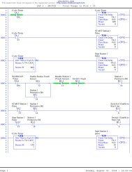
3. A program was written for the AT Mega32 that sets the PWM output and collects
data for the tachometer speed. The user inputs an integer between 0 and 9, which
sets the PWM output to a value between 0 and 255. The program begins to take
analog voltage input from the tachometer every 10 ms. When the user presses “t”
on the keyboard, the program generates a table that is displayed to the screen.
This program also includes compensation for deadband in the motor. The
program is shown in Appendix A.
4. The resistance of the motor was measured.
R = 9.4Ω
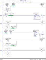
5. The motor and tachometer were wired to the AT Mega32 as shown in Figure 3.
5

Figure 3: Wiring diagram for AT Mega32 driving a motor with tachometer feedback
6. The deadband limits of the motor were measured using the program.
c_kinetic_posistve = 0x06
c_kinetic_negative = 0x12
c_static_positive = 0x07
c_static_negative = 0x08
7. From a previous lab activity, a relationship between the tachometer voltage and
the angular velocity was found to be:
⎛ 51⋅ π ⎞
ω = ⎜ ⎟ ⋅V
⎝ 30 ⎠
Also, the value of count must be converted to a voltage. This was accomplished
as follows:
V s
= count ⋅
5
255
8. Data was obtained for the values of count, V s , ω, K, τ, and J. The data is shown
in Table 1. The angular velocity of the tachometer is shown in Appendix B.
6

Discussion:
Count s
Table 1: Motor data
⎛ rad ⎞
ω ⎜ ⎟
⎝ sec ⎠
V (V)
K τ (sec)
2
J ( Kg ⋅ m )
28 0.55 515.38 0.00107 0.30 4.02E-07
56 1.10 696.67 0.00158 0.50 5.29E-07
84 1.65 766.09 0.00215 0.50 9.83E-07
112 2.20 805.56 0.00273 0.75 1.05E-06
140 2.75 821.87 0.00334 0.75 1.58E-06
168 3.29 832.56 0.00396 0.80 2.08E-06
196 3.84 841.16 0.00457 0.85 2.61E-06
224 4.39 848.28 0.00518 1.05 2.72E-06
252 4.94 863.12 0.00572 1.30 2.68E-06
The theoretical speed was calculated using Eq (11) with T = 0 . The equations used
were:
For count = 28
ω
( t)
= −
For count = 56
ω
( t)
= −
For count = 84
ω
( t)
= −
For count = 112
ω
( t)
For count = 140
ω
( t)
0.
55
0.
00107
1.
10
0.
00158
1.
65
0.
00215
⋅ e
⋅ e
⋅ e
2.
20
= − ⋅ e
0.
00273
2.
75
= − ⋅ e
0.
00334
⎛
−⎜
⎜
⎝
⎛
−⎜
⎜
⎝
⎛
−⎜
⎜
⎝
⎛
−⎜
⎜
⎝
⎛
−⎜
⎜
⎝
2
0.
00107
−7
4.
02 10
×
2
0.
00158
−7
5.
29 10
×
2
0.
00215
−7
9.
83 10
×
2
0.
00273
−6
1.
05 10
×
2
0.
00334
−6
1.
58 10
×
⎞
⎟⋅t
⎟
⎠
⎞
⎟⋅t
⎟
⎠
⎞
⎟⋅t
⎟
⎠
⎞
⎟⋅t
⎟
⎠
⎞
⎟⋅t
⎟
⎠
load
0.
55
+
0.
00107
1.
10
+
0.
00158
1.
65
+
0.
00215
2.
20
+
0.
00273
2.
75
+
0.
00334
7

For count = 168
ω
( t)
= −
For count = 196
ω
( t)
= −
For count = 224
ω
( t)
= −
For count = 252
ω
( t)
= −
3.
29
0.
00396
3.
84
0.
00457
4.
39
0.
00518
4.
94
0.
00572
⋅ e
⋅ e
⋅ e
⋅ e
⎛
−⎜
⎜
⎝
⎛
−⎜
⎜
⎝
⎛
−⎜
⎜
⎝
⎛
−⎜
⎜
⎝
2
0.
00396
−6
2.
08 10
×
2
0.
00457
−6
2.
61 10
×
2
0.
00518
−6
2.
72 10
×
2
0.
00572
−6
2.
68 10
×
⎞
⎟⋅t
⎟
⎠
⎞
⎟⋅t
⎟
⎠
⎞
⎟⋅t
⎟
⎠
⎞
⎟⋅t
⎟
⎠
3.
29
+
0.
00396
3.
84
+
0.
00457
4.
39
+
0.
00518
4.
94
+
0.
00572
The theoretical data for the angular velocity of the tachometer is shown in Appendix C.
The theoretical and experimental data for the various speeds were graphed. The graphs
are shown in Figures 4 through 12.
ω (rad/s)
600.00
500.00
400.00
300.00
200.00
100.00
Speed 1
0.00
0 200 400 600 800 1000 1200
Time (ms)
Experimental
Theoretical
Figure 4: Angular velocity (rad/sec) vs. Time (ms), with Count = 28
8

ω (rad/s)
800.00
700.00
600.00
500.00
400.00
300.00
200.00
100.00
Speed 2
0.00
0 200 400 600 800 1000 1200
Time (ms)
Experimental
Theoretical
Figure 5: Angular velocity (rad/sec) vs. Time (ms), with Count = 56
ω (rad/s)
900.00
800.00
700.00
600.00
500.00
400.00
300.00
200.00
100.00
Speed 3
0.00
0 200 400 600 800 1000 1200
Time (ms)
Experimental
Theoretcial
Figure 6: Angular velocity (rad/sec) vs. Time (ms), with Count = 84
9

ω (rad/s)
900.00
800.00
700.00
600.00
500.00
400.00
300.00
200.00
100.00
Speed 4
0.00
0 200 400 600 800 1000 1200
Time (ms)
Experimental
Theoretical
Figure 7: Angular velocity (rad/sec) vs. Time (ms), with Count = 112
ω (rad/s)
900.00
800.00
700.00
600.00
500.00
400.00
300.00
200.00
100.00
Speed 5
0.00
0 200 400 600 800 1000 1200
Time (ms)
Experimental
Theoretical
Figure 8: Angular velocity (rad/sec) vs. Time (ms), with Count = 140
10

ω (rad/s)
900.00
800.00
700.00
600.00
500.00
400.00
300.00
200.00
100.00
Speed 6
0.00
0 200 400 600 800 1000 1200
Time (ms)
Experimental
Theoretical
Figure 9: Angular velocity (rad/sec) vs. Time (ms), with Count = 168
ω (rad/s)
900.00
800.00
700.00
600.00
500.00
400.00
300.00
200.00
100.00
Speed 7
0.00
0 200 400 600 800 1000 1200
Time (ms)
Experimental
Theoretical
Figure 10: Angular velocity (rad/sec) vs. Time (ms), with Count = 196
11

ω (rad/s)
1000.00
900.00
800.00
700.00
600.00
500.00
400.00
300.00
200.00
100.00
Speed 8
0.00
0 200 400 600 800 1000 1200
Time (ms)
Experimental
Theoretical
Figure 11: Angular velocity (rad/sec) vs. Time (ms), with Count = 224
ω (rad/s)
1000.00
900.00
800.00
700.00
600.00
500.00
400.00
300.00
200.00
100.00
Speed 9
0.00
0 200 400 600 800 1000 1200
Time (ms)
Experimental
Theoretical
Figure 12: Angular velocity (rad/sec) vs. Time (ms), with Count = 252
12

To show the relationship between the applied voltage and angular acceleration, all nine
experimental speeds were graphed on a single graph. This is shown in Figure 13.
Conclusions:
ω (rad/s)
1000.00
800.00
600.00
400.00
200.00
0.00
Speeds 1 - 9
1 10 19 28 37 46 55 64 73 82 91 100
Time
Count 1
Count 2
Count 3
Count 4
Count 5
Count 6
Count 7
Count 8
Count 9
Figure 13: Angular velocity (rad/sec) vs. Time (ms) with speeds 1 – 9
• The experimental and theoretical data resulted in the same steady state angular
velocity.
• The theoretical data had a slightly slower acceleration than the experimental data.
o This was due to errors in the selection of τ for the theoretical data.
• The motor model is a very useful tool in the design and simulation of systems.
13

Appendix A – C Program
This program will set the PWM output and collect tachometer speed data. The user
inputs a number between 0 and 9, which sets the PWM to a value between 0 and 255.
The program will collect analog inputs every 10 ms. The data will be displayed onscreen
when “t” is pressed on the keyboard.
#include
#include
#include
#include "sio.c"
#define c_kinetic_pos 0x06 /* static friction */
#define c_kinetic_neg 0x12 /* make the value positive */
#define c_static_pos 0x07 /* kinetic friction */
#define c_static_neg 0x08 /* make the value positive */
#define c_max 255
#define c_min 255 /* make the value positive */
#define CLK_ms 50 /* update every 10 ms*/
int moving = 0; /* assume it starts without moving */
int j = 0;
int table[100];
int count = 0; /* a count value to be output on port B */
int db_correct = 1; /* deadband correction is on by default */
unsigned int CNT_timer0; /* The delay time */
volatile unsigned int CLK_ticks = 0; /* The current number of ms */
volatile unsigned int CLK_seconds = 0; /* The current number of seconds */
int deadband(int c_wanted);
void AD_setup();
int AD_read();
void PWM_init();
void PWM_update(int value);
int v_output(int v_adjusted);
void IO_setup();
void IO_update();
void delay(int ticks);
void create_array();
void CLK_setup();
int deadband(int c_wanted)
{ /* call this routine when updating */
int c_pos;
int c_neg;
int c_adjusted;
if(moving == 1)
{
c_pos = c_kinetic_pos;
c_neg = c_kinetic_neg;
14

}
}
else
{
c_pos = c_static_pos;
c_neg = c_static_neg;
}
if(c_wanted == 0)
{ /* turn off the output */
c_adjusted = 0;
}
else if(c_wanted > 0)
{ /* a positive output */
c_adjusted = c_pos +
(unsigned)(c_max - c_pos) * c_wanted / c_max;
if(c_adjusted > c_max) c_adjusted = c_max;
}
else
{ /* the output must be negative */
c_adjusted = -c_neg -
(unsigned)(c_min - c_neg) * -c_wanted / c_min;
if(c_adjusted < -c_min) c_adjusted = -c_min;
}
return c_adjusted;
void AD_setup()
{
ADMUX = 0xC0; // Set the input channel to zero
ADCSRA = 0xE0; // Turn on the ADC and set to free running
}
int AD_read()
{
return (ADCW >> 2); // Returns digital output from AD register
}
void PWM_init()
{ /* call this routine once when the program starts */
DDRD |= (1

{ /* call from the interrupt loop */
int RefSignal; // the value to be returned
if(v_adjusted >= 0)
{
/* set the direction bits to CW on, CCW off */
PORTC = (PINC & 0xFC) | 0x02; /* bit 1 on, 0 off */
if(v_adjusted > 255)
{ /* clip output over maximum */
RefSignal = 255;
}
else
{
RefSignal = v_adjusted;
}
}
else
{ /* need to reverse output sign */
/* set the direction bits to CW off, CCW on */
PORTC = (PINC & 0xFC) | 0x01; /* bit 0 on, 1 off */
if(v_adjusted < -255)
{ /* clip output below minimum */
RefSignal = 255;
}
else
{
RefSignal = -v_adjusted; /* flip sign */
}
}
}
return RefSignal;
void IO_setup()
{
DDRD = 0xFF; // all of port B is outputs
AD_setup(); // Enable AD inputs
PWM_init(); // Setup the PWM outputs
DDRA = (unsigned char)0; // Set port A to outputs
}
void IO_update()
{// This routine will run once per interrupt for updates
if(db_correct == 0)
{
PWM_update(v_output(count));
}
else
{
PWM_update(v_output(deadband(count)));
}
if(count > 0)
{
create_array();
}
}
16

void delay(int ticks)
{ // ticks are approximately 1ms
volatile int i, j;
}
for(i = 0; i < ticks; i++)
{
for(j = 0; j < 1000; j++){}
}
SIGNAL(SIG_OVERFLOW0)
{ // The interrupt calls this function
}
CLK_ticks += CLK_ms;
if(CLK_ticks >= 10)
{ // The number of interrupts between output changes
CLK_ticks = CLK_ticks - 10;
CLK_seconds++;
IO_update();
}
TCNT0 = CNT_timer0;
void CLK_setup()
{ // Start the interrupt service routine
}
TCCR0 = (0

}
{
}
j = 0;
count = 0;
// -------------- The main program loop ------------------
int main()
{
int c;
sio_init();
IO_setup();
CLK_setup();
for(;;)
{
while((c = input()) == -1){} // wait for a keypress
if(c == 'd')
{
if(db_correct == 0)
{
db_correct = 1;
outln("Deadband correction on");
}
else
{
db_correct = 0;
outln("Deadband correction off");
}
}
else if(c == 's')
{
count = 0;
moving = 0;
outint(count);
outln(" = count, motor stopped");
}
else if(c == 'h')
{
outln(" d: enable (default) or disable deadband comp.");
outln(" s: stop the motor");
outln(" q: quit");
}
else if(c == '0')
{
count = 0;
}
else if(c == '1')
{
count = 28;
}
else if(c == '2')
{
count = 56;
}
18

}
sio_cleanup();
return 1;
}
else if(c == '3')
{
count = 84;
}
else if(c == '4')
{
count = 112;
}
else if(c == '5')
{
count = 140;
}
else if(c == '6')
{
count = 168;
}
else if(c == '7')
{
count = 196;
}
else if(c == '8')
{
count = 224;
}
else if(c == '9')
{
count = 252;
}
else if(c == 'r')
{
count = 0;
outln("stopped");
j = 0;
}
else if(c == 't')
{
int k;
for(k = 0; k < 100; k++)
{
outint(table[k]);
outln("");
}
}
else if(c == 'q')
{
count = 0;
moving = 0;
outint(count);
outln(" = count, Quitting");
break;
}
19

Appendix B – Experimental angular velocity
20

Appendix C – Theoretical angular velocity
22