- Page 1 and 2:
sBuipaaoojd paj.sgsse-ja).nduioo uo
- Page 3 and 4:
of the international symposium on c
- Page 5 and 6:
PREFACE The. te.chnic.at oAticJteA
- Page 7:
Seminar on Statistical Mapping . .
- Page 11 and 12:
CHARGE TO THE CONFERENCE William B.
- Page 13:
CONCLUSION Summing up, the introduc
- Page 17 and 18:
INTRODUCTION MAP DESIGN Arthur H. R
- Page 19 and 20:
Because it will help to emphasize a
- Page 21 and 22:
The main idea behind the communicat
- Page 23 and 24:
INTRODUCTION A CHALLENGE TO CARTOGR
- Page 25 and 26:
manner: The authors have attempted
- Page 27 and 28:
But just how new is the concept of
- Page 29 and 30:
Clearly the ability and the desire
- Page 31 and 32:
The third step is the DECISION stag
- Page 33 and 34:
He went on to call for the creation
- Page 35 and 36:
VISIONS OF MAPS AND GRAPHS William
- Page 37 and 38:
intution, rule of thumb, and a kind
- Page 39 and 40:
(Of course it might be that some ca
- Page 41 and 42:
How stable, for example, are the re
- Page 43 and 44:
Henry ¥ Castner and Arthur H. Robi
- Page 45 and 46:
General Session Papers Introduction
- Page 47 and 48:
WALP0 T08LER has been with the. Geo
- Page 49 and 50:
INTRODUCTION A GEOGRAPHIC AND CARTO
- Page 51 and 52:
In addition, numerous administrativ
- Page 53 and 54:
DELINEATION OF STATISTICAL AREAS Su
- Page 55 and 56:
which exist around the central citi
- Page 57 and 58:
distribution of school children by
- Page 59 and 60:
INTRODUCTION CONTEMPORARY STATISTIC
- Page 61 and 62:
tial relationships of cropland acre
- Page 63 and 64:
Figures 3 and k. At least part of w
- Page 65 and 66:
AESTHETICS AND MAP COMMUNICATION Th
- Page 67 and 68:
As a case in point, study the three
- Page 69 and 70:
ABSTRACT CHARACTER OF A MAP TOPOLOG
- Page 71 and 72:
epresents the operator composition
- Page 73 and 74:
Thus a contour lies between two of
- Page 75 and 76:
(2) From this table compute plane c
- Page 77 and 78:
4: A Topogtuipkic. 1970 POPULRTION
- Page 79 and 80:
county map of the United States has
- Page 81 and 82:
If. D. Kendall, "Construction Of Ma
- Page 83 and 84:
By the way, graphs used for the var
- Page 85 and 86:
c. Suppose that maps are constructe
- Page 87 and 88:
Graph2: MEDIAN INCOME IN 1949 OF FA
- Page 89 and 90:
adults (see Yule and Kendall, 1950,
- Page 91 and 92:
original GRP, and a scale of tens h
- Page 93 and 94:
them (or in semi-logarithmic charts
- Page 95 and 96:
(iiaphll USA (1840, 1900, I960) Per
- Page 97 and 98:
ooooooooooooo< 4 DD 4 D 4 C 4 ooooo
- Page 99 and 100:
INTRODUCTION THE CHALLENGE OF MAPS
- Page 101 and 102:
Gilligan and Amendola here in the U
- Page 103 and 104:
handicapped will be better served b
- Page 105 and 106:
REFERENCES 1. Professor James F. Go
- Page 107 and 108:
INTRODUCTION MAP GENERALIZATION: TH
- Page 109 and 110:
map, symbols can be assigned and th
- Page 111 and 112:
that simplification of lines result
- Page 113 and 114:
Map 3a. .01 Map 3b. .30 Map 3c. .60
- Page 115 and 116:
75,000
- Page 117 and 118:
As mentioned earlier, most surface
- Page 119 and 120:
exponentially with the number of po
- Page 121 and 122:
Panel Discussion on Experiences in
- Page 123 and 124:
C. GENE JOHNSON iA chie.fi ofi the.
- Page 125 and 126:
And in talking about the possibilit
- Page 127 and 128:
INTRODUCTION DECISION DAY FOR AUTOM
- Page 129 and 130:
THE ORDNANCE SURVEY This organizati
- Page 131 and 132:
AUTOMATED CARTOGRAPHY AT THE U. S.
- Page 133 and 134:
Two steps of choropleth mapping hav
- Page 135 and 136:
The identification subsystem will u
- Page 137 and 138:
AUTOMATED CARTOGRAPHY IN THE NATION
- Page 139:
GEODETIC CONTROL MAPS The National
- Page 142 and 143:
SEMINAR ON STATISTICAL MAPPING This
- Page 144 and 145:
INTRODUCTION STATISTICAL ACCURACY A
- Page 146 and 147:
was purposely conventional. The low
- Page 148 and 149:
F;VL - FIVE 7 FIVE 9 FIVE M FIVE 16
- Page 150 and 151:
classes tended to smooth out the bl
- Page 152 and 153:
TABLE III. OVERALL ACCURACY OF THE
- Page 154 and 155:
epresentation of statistical relati
- Page 156 and 157:
7. G. Jenks and F. Caspall, "Error
- Page 158 and 159:
7. A -6eo£con oft the. UrUte,d Sta
- Page 160 and 161:
3. Two boie map* pAepaAed tfoA paAt
- Page 162 and 163:
Figure 5 are generalizations of the
- Page 164 and 165:
City Selection The twenty largest m
- Page 166 and 167:
Dot distribution maps are used for
- Page 168 and 169:
plate. Pages with isopleth maps and
- Page 170 and 171:
THE URBAN ATLAS PROJECT: HISTORICAL
- Page 172 and 173:
The feasibility of such a project,
- Page 174 and 175:
SCALE Since the primary purpose of
- Page 176 and 177:
LINE-WEIGHT The line-weight of the
- Page 178 and 179:
SEMINAR ON MAP REAPING ANV PERCEPTI
- Page 180 and 181:
perception using the. basic oAAumpt
- Page 182 and 183:
an attempt to reach a re.atistic mo
- Page 184 and 185:
Census of Agriculture, the Census B
- Page 186 and 187:
maps. Research cartographers have m
- Page 188 and 189:
Five shades in black and white or c
- Page 190 and 191:
Ve selected this scheme for use in
- Page 192 and 193:
The important shift that has occurr
- Page 194 and 195:
For a good many years, researchers
- Page 196 and 197:
So far cartographic research in map
- Page 198 and 199:
This will be a difficult order, eve
- Page 200 and 201:
This is equally true of many aspect
- Page 202 and 203:
AN ANALYSIS OF APPROACHES IN MAP DE
- Page 204 and 205:
the clues that you get in the visua
- Page 206 and 207:
take immediate action to correct th
- Page 208 and 209:
• BASE MAPS PLANIMETRIC TOPOGRAPH
- Page 210 and 211:
as the one in the front of the room
- Page 212 and 213:
INTRODUCTION CURRENT RESEARCH IN TA
- Page 214 and 215:
D.B.RH. NEIGHBORHOOD MAP Key ;to m
- Page 216 and 217:
3. GENERAL REFERENCE MAP OF THE UNI
- Page 218 and 219:
tions were noted for both practiced
- Page 220 and 221:
for the single lines, ranging from
- Page 222 and 223:
INTRODUCTION THE OPTIMAL THEMATIC M
- Page 224 and 225:
eye comes to rest for at least 2/10
- Page 226 and 227:
The 20 reconstructed maps were then
- Page 228 and 229:
307 302 Figure. 10. TkeAe. two tKLc
- Page 230 and 231:
~i 12. The^e, dote -6how the. locat
- Page 233 and 234:
INTRODUCTION THE MAP IN THE MIND'S
- Page 235 and 236:
VALUE OF RETAIL TRADE SURPLUS LOCAT
- Page 237 and 238:
has a prominent role in goal specif
- Page 239:
the subjects some elements are domi
- Page 242 and 243:
a sound explanation for it. A secon
- Page 244 and 245:
Finally, one of the most interestin
- Page 246 and 247:
INTRODUCTION IN PURSUIT OF THE MAP
- Page 248 and 249:
producing a personal image fictitio
- Page 250 and 251:
individuals chosen appear from the
- Page 252 and 253:
screen gray area and its perceived
- Page 254 and 255:
There are a number of questions whi
- Page 256 and 257:
Note, first, that the four areas wi
- Page 258:
18. Stevens, S.S. (Geraldine Steven
- Page 261 and 262:
PER CAPITA INCOME: 1 970 3.
- Page 263 and 264:
MICROFILM OUTPUT This film is a typ
- Page 265 and 266:
ANAHEIM-SANTA ANA- GARDEN GROVE, CA
- Page 267 and 268:
ANAHEIM-SANTA ANA- GARDEN GROVE, CA
- Page 269 and 270:
NUMBER OF AMERICAN INDIANS COUNTIES
- Page 271 and 272:
HOUSING UNITS BUILT BEFORE 1950 - W
- Page 273 and 274:
NESTED CATEGORIES EMPHASIS ON EXTRE
- Page 275 and 276:
Seminar on Uses of Color Introducti
- Page 277 and 278:
In theJji pne*entation f "Tke- Sele
- Page 279 and 280:
INFORMATION PROCESSING AND RECALL T
- Page 281 and 282:
The great 19th century physicist Ja
- Page 283 and 284:
general, there is a tendency for a
- Page 285 and 286:
THE SELECTION OF COLOR FOR THE U.S.
- Page 287 and 288:
mixes for CIA with the formulas on
- Page 289 and 290:
Red Cyan Yellow Other Color Agrocli
- Page 291 and 292:
Red Cyan Yellow Other Color Rural P
- Page 293 and 294:
Administrative Divisions, p. 58 —
- Page 295 and 296:
spaced in hue, such as this sequenc
- Page 297 and 298:
THE ORGANIZATION OF COLOR ON TWO-VA
- Page 299 and 300:
diagonal. (See Figure 18, page 265
- Page 301 and 302:
CONCLUDING COMMENTS Finally, there
- Page 303 and 304:
Seminar on Automation in Cartograph
- Page 305 and 306:
The. majoA tkAaAt o& the. TopogAaph
- Page 307 and 308:
Subcontracted work has until now ge
- Page 309 and 310:
Software development before 1970 di
- Page 311 and 312:
INTRODUCTION INTERACTIVE CARTOGRAPH
- Page 313 and 314: Our system assumes that automated c
- Page 315 and 316: can be taught to correct some, at l
- Page 317 and 318: this, very little attempt has been
- Page 319 and 320: The vast increase in speed (about t
- Page 321 and 322: Data Management System 1100 (now us
- Page 323 and 324: APPENDIX B: A BRIEF DISCUSSION OF H
- Page 325 and 326: CO-ORDINATE SYSTEMS AND TRANSFORMS
- Page 327 and 328: A digital data bank comprises colle
- Page 329 and 330: The second advantage is particularl
- Page 331 and 332: The production of maps, however, re
- Page 333 and 334: Things become more complicated with
- Page 335 and 336: For less high quality we plan to el
- Page 337: One of the most important facts in
- Page 340 and 341: SEMINAR ON AUTOMATION IN CARTOGRAPH
- Page 342 and 343: pAoje,ct at the. LaboAatoAy fioA Co
- Page 344 and 345: Master Enumeration District List (M
- Page 346 and 347: as seen in Figure 1. The resulting
- Page 348 and 349: (X). Implicitly this problem is ide
- Page 350 and 351: 6. Fou/i data. po^ntA loc.at
- Page 352 and 353: F-tgote 7. Cteecf and open Thxte64e
- Page 354 and 355: INTRODUCTION TOPOLOGICAL INFORMATIO
- Page 356 and 357: Topological notation emphasizes the
- Page 358 and 359: NEW PROCEDURES In particular, many
- Page 360 and 361: -INTRODUCTION CONTOURING ALGORITHMS
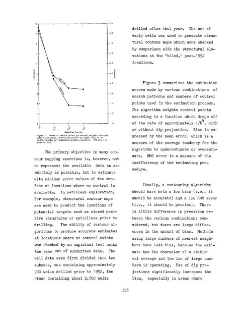
- Page 362 and 363: The second step is the estimation o
- Page 366 and 367: obtainable. An algorithm which fait
- Page 369 and 370: Seminar on Land Use Mapping Introdu
- Page 371 and 372: de.veJtopme.nt and availability ofi
- Page 373 and 374: Image. pAocessing te.chniqu.eA oAig
- Page 375 and 376: INTRODUCTION LAND UNIT MAPPING WITH
- Page 377 and 378: MANAGEMENT COMPONENTS • Highly de
- Page 379 and 380: SOURCE MAP CHARACTERISTICS WRIS has
- Page 381 and 382: Polygon boundaries to be digitized
- Page 383 and 384: less than 10 minutes. This speed wi
- Page 385 and 386: 6. Diello, Joseph, (1970), The Evol
- Page 387 and 388: the map is only peripheral at prese
- Page 389 and 390: THE NATURE OF PROPERTY TAXATION TAX
- Page 391 and 392: The maps are actually parts of an i
- Page 393 and 394: 5. Commonwealth of Massachusetts, D
- Page 395 and 396: LANDSAT image, a stereoscopic pair
- Page 397 and 398: The climate of the area is moderate
- Page 399 and 400: The developed formula of peak runof
- Page 401 and 402: This coordinate system is shown on
- Page 403 and 404: The drainage basin maps show the ac
- Page 405 and 406: BLOCK #24-21 (continued) 3. 153 Del
- Page 407 and 408: SQUARE 2 1 ^ i 7 2 —— ~1T ~6^ 8
- Page 409 and 410: 24-21 msv -Co 75° 12' 40° 38' X =
- Page 411 and 412: 24-21 75°I2' 40°38' X = 1851968.7
- Page 413 and 414: 24-21 75° I2 1 40°38 X= 1851968.
- Page 415 and 416:
BRIEF ANALYSIS OF THE USERS The req
- Page 417:
6. Halasi-Kun, G. J. (1975), "Water
- Page 420 and 421:
SEMINAR ON IWTERACTIl/E MAP EPITING
- Page 422 and 423:
0/ES SHEPHERD o$ the. U.S. Amy Engi
- Page 424 and 425:
Youngmann (1972), Peucker (1973)> a
- Page 426 and 427:
developed in other areas, to the so
- Page 428 and 429:
7. Christian!, E. J., et al., 1973>
- Page 430 and 431:
NEIGHBORHOODS MAP EDITING USING A T
- Page 432 and 433:
FUTURE RESEARCH Every field in a DI
- Page 434 and 435:
3. "Hie fiundanuintal noA.Qkbonhood
- Page 436 and 437:
7. Tkn dua£ $fw.pk aA.ou.nd ueA^ex
- Page 438 and 439:
INTRODUCTION GDIS VS. CUE: A LOOK A
- Page 440 and 441:
3. Douglas County Auto Title/Regist
- Page 442 and 443:
3. The lack of broad based local go
- Page 444 and 445:
that intergovernmental cooperation
- Page 446 and 447:
2. Inquiry by address - The fields
- Page 448 and 449:
cities throughout the United States
- Page 450 and 451:
REQUEST 1 DIME FILE RECORD U P D A
- Page 452 and 453:
REQUEST 3 DIME RES P 0 N S E S C R
- Page 454 and 455:
REQUEST 7 DIME RE S P 0 N S E S C R
- Page 456 and 457:
INTRODUCTION AN INTERACTIVE GBF CRE
- Page 458 and 459:
equiring a GBF in a slightly differ
- Page 461 and 462:
Seminar on Urban Information System
- Page 463 and 464:
1/ICT0R PA I/IS oi the. Ci£y ojj A
- Page 465 and 466:
INTRODUCTION ANALYTICAL MAPS FOR SC
- Page 467 and 468:
coordinates (referred to as rectili
- Page 469 and 470:
The map of Figure 3 shows the bound
- Page 471 and 472:
Figure 4 BLACK STUDENT ASSIGNMENTS:
- Page 473 and 474:
Maps based on student-allocation mo
- Page 475 and 476:
housing development per every stude
- Page 477 and 478:
COMPUTER MAPPING AND ITS IMPACT ON
- Page 479 and 480:
the shades. Digit 5 is a coded numb
- Page 481 and 482:
The most frequent use of computer m
- Page 483 and 484:
\ \ / ,.L5_i / /hjgj-->-»• VJ1 .
- Page 485 and 486:
B g TM BT BSTH TER M B8TH TfH M SBT
- Page 487 and 488:
GRAFPAC Subroutines ADVANG - ADVANG
- Page 489 and 490:
TABDVG - TABDVG initializes that pa
- Page 491 and 492:
several decades increasing amounts
- Page 493 and 494:
Automated Evolution of the Time Fac
- Page 495 and 496:
It merits noting that operators and
- Page 497 and 498:
So as to be consistent with the pre
- Page 499 and 500:
INTRODUCTION GEOLOGICAL INFORMATION
- Page 501 and 502:
or values (weights) to the presence
- Page 503 and 504:
factors are depicted in shades of g
- Page 505 and 506:
Proper use of UNIMATCH, however, fr
- Page 507 and 508:
INTRODUCTION THE CONGRUENCE BETWEEN
- Page 509 and 510:
By 1968 SACS had been conceptually
- Page 511 and 512:
in an engineering precision. Inhere
- Page 513 and 514:
Seminar on Data Structures Introduc
- Page 515 and 516:
*cheme* oft aggregation present and
- Page 517 and 518:
(Clement, 197*0> etc., have all bee
- Page 519 and 520:
A line of n points can be subdivide
- Page 521 and 522:
LINE GENERALIZATION The theory of t
- Page 523 and 524:
shortened to close to half by const
- Page 525 and 526:
DOUBLE LINE AND OTHER LINE SYMBOLS
- Page 527 and 528:
INTRODUCTION APPLICATIONS OF LATTIC
- Page 529 and 530:
The computation of intersections is
- Page 531 and 532:
CARTOGRAPHIC DATA BASE DESCRIPTION
- Page 533 and 534:
Cartographic data for the United St
- Page 535 and 536:
P/iopo-i ecf D M S Output Decimal S
- Page 537 and 538:
BASE CATEGORY IV - TERRAIN SURFACE
- Page 539 and 540:
objectives of a specific data base.
- Page 541 and 542:
COORDINATE POINT DIRECTORY Coord. 4
- Page 543 and 544:
7\ POINTS Ident. (Name) CHAIN GROUP
- Page 545 and 546:
Some of the attributes of a topolog
- Page 547 and 548:
Seminar on Automation in Cartograph
- Page 549 and 550:
infrastructure, and human resources
- Page 551 and 552:
negative and repel each other. This
- Page 553 and 554:
THE GRIMAS SYSTEM APPLICATION softw
- Page 555 and 556:
GRIMAS SYSTEM FLOW: PLOT -CONTROL/
- Page 557 and 558:
All object classes have locational
- Page 559 and 560:
PROJECT BAR CHART TR M E S T E R RR
- Page 561 and 562:
To get a flexible system it was dec
- Page 563 and 564:
E. - Topography 80 Man-Hours F. - G
- Page 565 and 566:
The goal described above is further
- Page 567 and 568:
1. With respect to the dimensional
- Page 569 and 570:
561 BRRSIL FUNDRCRO I.B.G.E. DIRETO
- Page 571 and 572:
SPECIAL AND THEMATIC MAP SERIES The
- Page 573 and 574:
As to geodetics and topography, the
- Page 575 and 576:
THE AIR FORCE MINISTRY: ELECTRONICS
- Page 577:
URBAN AND RURAL, TECHNICAL AND FISC
- Page 580 and 581:
APPENDIX I AUTO-CARTO II STAFF AND
- Page 582 and 583:
Robert T. Aangeenbrug Department of
- Page 584 and 585:
H. G. Barnum University of Vermont
- Page 586 and 587:
Kurt E. Brassel Assistant Professor
- Page 588 and 589:
James M. Collom Cartographer NOAA N
- Page 590 and 591:
James F. Dixon Assistant Director G
- Page 592 and 593:
John B. Fieser Program Specialist U
- Page 594 and 595:
Terry W. Gossard U.S.D.A. Forest Se
- Page 596 and 597:
Daniel E. Holdgreve 507 Kibler Circ
- Page 598 and 599:
Olaf Kays Asst. Program Mgr.-RALI U
- Page 600 and 601:
Gary Lewis Graphics Coordinator Tet
- Page 602 and 603:
S. E. Masry Assoc. Professor Univer
- Page 604 and 605:
David C. Mowbray Head, Map Informat
- Page 606 and 607:
Thomas K, Peucker Assoc. Prof. , Si
- Page 608 and 609:
William R. Roseman Vice President I
- Page 610 and 611:
Lee Henry Slorp Miami University, D
- Page 612 and 613:
G. L. Thornton Research and Develop
- Page 614 and 615:
Dean P. Westmeyer Cartographic Edit
- Page 616 and 617:
APPENDIX III AUTHOR AND TITLE INDEX
- Page 618 and 619:
Contemporary Statistical Map6: Evid
- Page 620 and 621:
Martell, Alberto Torfer (Automation
- Page 622:
Van Driel, Nicholas (Ge.ological In