Gauge theory for embedded surfaces, II

More documents

Recommendations

Info

$Math 126 Solution Set 2$

$Math S?101. Worksheet 1. Axioms of Integer Arithmetic$

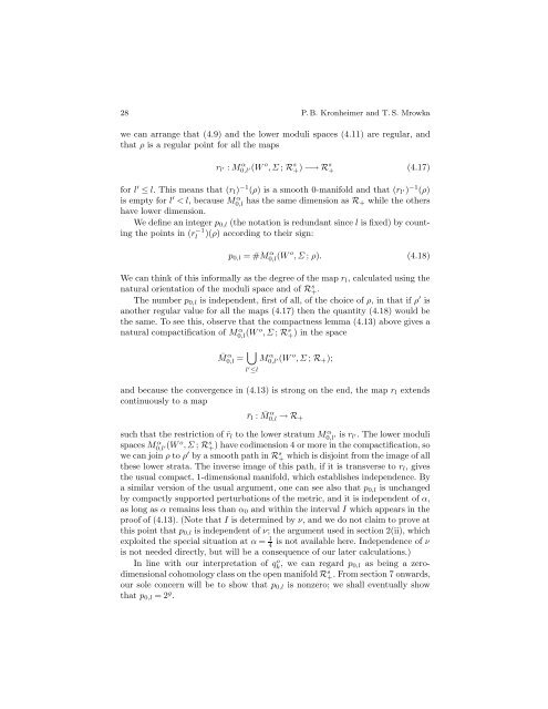
28 P. B. Kronheimer and T. S. Mrowka we can arrange that (4.9) and the lower moduli spaces (4.11) are regular, and that ρ is a regular point for all the maps rl ′ : M α 0,l ′(W o ,Σ; R s + )−→ Rs + (4.17) for l ′ ≤ l. This means that (rl) −1 (ρ) is a smooth 0-manifold and that (rl ′)−1 (ρ) is empty for l ′
Gauge theory for embedded surfaces, II 29 5. The main excision argument Having defined invariants associated with manifolds with cylindrical ends in the previous section, we shall now use the gluing results to show how these combine to give the invariants qk and qk,l for the closed manifold X and the pair (X,Σ) respectively. The end result is our excision principle, that the difference between qk and qk,l can be calculated from data which is associated only with the neighbourhood of Σ. We shall also use part of the same argument to prove another key result, a vanishing theorem in part (iii). (i) The gluing formula for qk,l. Let (X,Σ) again be an acceptable pair, with X simply connected. We shall suppose that the genus and self-intersection number of Σ satisfy the inequality of Condition 4.1, so that the invariants qo k are defined for the cylindrical end space Xo . We shall also assume, as in section 4(ii), that the genus is odd, and we add an extra hypothesis, that the self-intersection number n is not divisible by 4 (this will be used in the proof of (5.5) below). We again set l = 1 4 (2g − 2) (4.10), so the invariant p0,l is defined from the moduli space on W o . Fix an integer k and let d be given, as usual, by (4.2). We suppose these are in the ‘stable range’, so 2d>4k. Proposition 5.1. Under the above hypotheses, the invariant qk,l of the pair (X,Σ) can be calculated in terms of the invariants q o k and p0,l associated with the cylindrical end spaces by the formula qk,l(u1,...,ud)=p0,lq o k(u1,...,ud), for all homology classes u1,...,ud in H2(X\Σ). Proof. Recall first that p0,l is defined using a moduli space with a small value of α. Precisely, we choose a value of α less than the α0 given in (4.15), we choose a compact interval I containing α, and we then choose the cone parameter ν to be sufficiently large that the conclusion of Proposition 2.12 holds (see the proof of (4.13) above). Fixing such parameters, we introduce the temporary abbreviation M α 0,l (W o ) for the moduli space (4.9), and M α 0,l ′(W o )forthelower moduli spaces (4.11). We denote by rl and rl ′ the maps to Rs +. We assume that the moduli spaces are regular, so the invariant p0,l is calculated as the ‘degree’ of rl at any ρ which is a regular value of all the rl ′. Let K be the moduli space from Xo , cut down by the subvarieties associated with the ui: K(X o )=Mk(X o ;R s + )∩V1∩...∩Vd. (5.2) We choose the metric on X o and the sections defining the Vi so that this space, as well as the lower spaces (4.4), are all regular. In addition, we arrange that the map rX : K(X o ) −→ R s +
Page 1 and 2: Gauge theory for embedded surfaces,
Page 27: Gauge theory for embedded surfaces,

Gauge theory for embedded surfaces, II

Create successful ePaper yourself

Delete template?

Save as template?