LMI Approach to Iterative Learning Control Design - ResearchGate

More documents

Recommendations

Info

In this paper we show that the LMI method can be used to design the optimal ILC learning gain matrix. The paper is organized as follows. The super-vector ILC structure is analyzed in Section II Based on the analysis of Section II, LMI algorithms are designed in Section III and LMI test results are shown in Section IV. Conclusions are given in Section V. II. 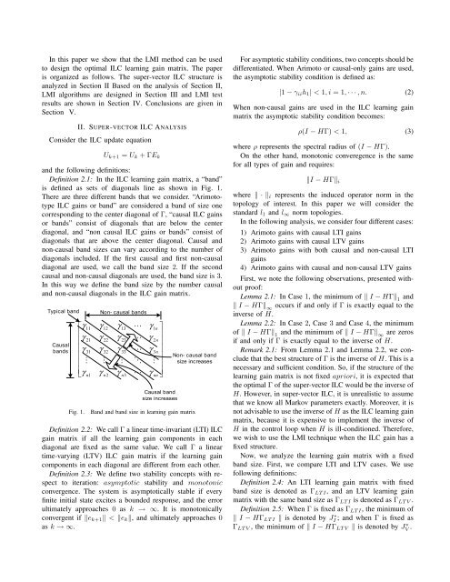SUPER-VECTOR ILC ANALYSIS Consider the ILC update equation Uk+1 = Uk + ΓEk and the following definitions: Definition 2.1: In the ILC learning gain matrix, a “band” is defined as sets of diagonals line as shown in Fig. 1. There are three different bands that we consider. “Arimototype ILC gains or band” are considered a band of size one corresponding to the center diagonal of Γ, “causal ILC gains or bands” consist of diagonals that are below the center diagonal, and “non causal ILC gains or bands” consist of diagonals that are above the center diagonal. Causal and non-causal band sizes can vary according to the number of diagonals included. If the first causal and first non-causal diagonal are used, we call the band size 2. If the second causal and non-causal diagonals are used, the band size is 3. In this way we define the band size by the number causal and non-causal diagonals in the ILC gain matrix. Typical band Causal bands ⎡γ ⎢ ⎢ γ ⎢γ ⎢ ⎢ M ⎢ ⎣γ n 11 21 31 1 γ γ γ γ Non- causal bands 12 22 32 M n2 γ γ γ γ 13 23 33 M n3 L L L O L γ 1n ⎤ γ ⎥ 2n ⎥ γ ⎥ 3n ⎥ M ⎥ γ ⎥ nn ⎦ Causal band size increases Non- causal band size increases Fig. 1. Band and band size in learning gain matrix Definition 2.2: We call Γ a linear time-invariant (LTI) ILC gain matrix if all the learning gain components in each diagonal are fixed as the same value. We call Γ a linear time-varying (LTV) ILC gain matrix if the learning gain components in each diagonal are different from each other. Definition 2.3: We define two stability concepts with respect to iteration: asymptotic stability and monotonic convergence. The system is asymptotically stable if every finite initial state excites a bounded response, and the error ultimately approaches 0 as k → ∞. It is monotonically convergent if ek+1 < ek, and ultimately approaches 0 as k → ∞. For asymptotic stability conditions, two concepts should be differentiated. When Arimoto or causal-only gains are used, the asymptotic stability condition is defined as: |1 − γiih1| < 1, i = 1, · · · , n. (2) When non-causal gains are used in the ILC learning gain matrix the asymptotic stability condition becomes: ρ(I − HΓ) < 1, (3) where ρ represents the spectral radius of (I − HΓ). On the other hand, monotonic converegence is the same for all types of gain and requires: I − HΓi where · i represents the induced operator norm in the topology of interest. In this paper we will consider the standard l1 and l∞ norm topologies. In the following analysis, we consider four different cases: 1) Arimoto gains with causal LTI gains 2) Arimoto gains with causal LTV gains 3) Arimoto gains with both causal and non-causal LTI gains 4) Arimoto gains with causal and non-causal LTV gains First, we note the following observations, presented without proof: Lemma 2.1: In Case 1, the minimum of I − HΓ1 and I − HΓ∞ occurs if and only if Γ is exactly equal to the inverse of H. Lemma 2.2: In Case 2, Case 3 and Case 4, the minimum of I − HΓ1 and the minimum of I − HΓ∞ are zeros if and only if Γ is exactly equal to the inverse of H. Remark 2.1: From Lemma 2.1 and Lemma 2.2, we conclude that the best structure of Γ is the inverse of H. This is a necessary and sufficient condition. So, if the structure of the learning gain matrix is not fixed apriori, it is expected that the optimal Γ of the super-vector ILC would be the inverse of H. However, in super-vector ILC, it is unrealistic to assume that we know all Markov parameters exactly. Moreover, it is not advisable to use the inverse of H as the ILC learning gain matrix, because it is expensive to implement the inverse of H in the control loop when H is ill-conditioned. Therefore, we wish to use the LMI technique when the ILC gain has a fixed structure. Now, we analyze the learning gain matrix with a fixed band size. First, we compare LTI and LTV cases. We use following definitions: Definition 2.4: An LTI learning gain matrix with fixed band size is denoted as ΓLT I, and an LTV learning gain matrix with the same band size as ΓLT I is denoted as ΓLT V . Definition 2.5: When Γ is fixed as ΓLT I, the minimum of I − HΓLT I is denoted by J ∗ I ; and when Γ is fixed as ΓLT V , the minimum of I − HΓLT V is denoted by J ∗ V .
Then, using Definition 2.4 and Definition 2.5, we have following theorem, also stated without proof, from the fact that ΓLT I ⊂ ΓLT V . Theorem 2.1: If the same band size ILC gain matrices are used in ΓLT I and ΓLT V , the following inequality is satisfied: J ∗ V ≤ J ∗ I Remark 2.2: Theorem 2.1 relates the optimality between Case-1 and Case-2 and the optimality between Case-3 and Case-4. Also, from Theorem 2.1, the following corollary is immediate. Corollary 2.1: If the same band size is used in causal ILC and non-causal/causal ILC, then J ∗ N ≤ J ∗ C, where J ∗ N is the minimum value using causal, Arimoto, and non-causal learning gains; and J ∗ C is the minimum value using only causal and Arimoto gains. In summary, from Lemma 2.1 and Lemma 2.2, we conclude that the best gain matrix is just the inverse of H with respect to convergence in the l1 and l∞ norms. When the band size is fixed, we conclude that LTV is better than LTI from Theorem 2.1, and from Corollary 2.1 that including non-causal terms increases the optimality of the system. III. LMI DESIGN In this section, we show how to use LMI techniques for ILC design using several different fixed ILC gain matrix structures. Suppose we wish to satisfy the monotonic convergence condition min[σ(I − HΓ)]. Now, because and because: σ[I − HΓ] ≡ λ([I − HΓ][I − HΓ] T ). λ([I − HΓ][I − HΓ] T ) ≤ [I − HΓ][I − HΓ] T then by minimizing [I − HΓ][I − HΓ] T , we can limit the upper bound of σ(I − HΓ). Because min( [I − HΓ][I − HΓ] T ) is a typical matrix inequality problem, the ILC design problem can thus be solved by an LMI. We consider three cases: 1. LMI − 1: Not-fixed learning gain matrix In LMI − 1, we do not fix the gain matrix structure, and the LMI algorithm finds the best structure by minimizing I − HΓ using Γ. A typical LMI is designed as subject to max{−x 2 1} x 2 1In×n > [I − HΓ][I − HΓ] T . (4) However, (4) is a quadratic form, so we change (4) to a linear inequality form given by x1In×n [I − HΓ] [I − HΓ] T > 0 (5) x1In×n The more simplified form is designed according to −x2 0 In×n H 1I2n×2n − + Γ [ 0 In×n ] In×n 0 0 0 + ΓT [ HT 0 ] < 0. (6) In×n Then x1 is an optimization scalar variable and Γ is an optimization matrix variable. 2. LMI − 2: LTI ILC with fixed band size As shown in Fig. 2.2 in the next section, the LMI algorithm finds the inverse of H as the optimal gain. This is already an expected result from the analysis of Section II. So, in this case, a big band-size gain matrix is indispensable. However, as already commented, the big band-size gain matrix is not practical. Thus, we design using LMIs by forcing a fixed gain matrix structure as shown in Fig. 1. For convenience, we use following learning gain matrix notation: ⎡ ⎢ Γ = ⎢ ⎣ γp γ1 N γ2 N · · · γ n−1 N γ1 C γp γ1 N · · · γ n−2 N γ2 C γ1 C γp · · · γ n−3 N . .. . γ n−1 C . γ n−2 C . γ n−3 C · · · γp . ⎤ ⎥ ⎦ , where subscripts C, p, and N mean causal, Arimoto (proportional terms), and non-causal gains, respectively. The total number of variables in the learning gain matrix is 2n − 1. As already explained, if only γp is used in Γ, the band size is 1; if γp, γ1 C , and γ1 N are used, the band size is 2, and in the same way, if γp, γ 1 C ,· · ·,γk C , and γ1 N ,· · ·,γk N are used, the band size is k + 1. To design a linear LMI, we change I − HΓ to In×n − [γ n−1 C Hn−1 C + · · · + γ1 CH1 C + γpHp + · · · + γn−1 ], (7) +γ 1 N H1 N N Hn−1 N where Hk C , k = 1, · · · , n−1 are Markov matrices corresponding to causal gains; Hp is a Markov matrix corresponding to Arimoto gains; and Hk N , k = 1, · · · , n − 1 are Markov matrices corresponding to non-causal gains. For example, they are expressed as: H 1 ⎡ 0 0 0 · · · ⎤ 0 ⎢ C = ⎢ ⎣ h1 h2 . 0 h1 . 0 0 . · · · · · · . .. 0 ⎥ 0 ⎥ . ⎦ hn−1 hn−2 hn−3 · · · 0
Page 1: LMI Approach to Iterative Learning
Page 5 and 6: TABLE III ALGORITHMS FOR LMI CONSTR

LMI Approach to Iterative Learning Control Design - ResearchGate

Create successful ePaper yourself

Delete template?

Save as template?