LMI Approach to Iterative Learning Control Design - ResearchGate
LMI Approach to Iterative Learning Control Design - ResearchGate
LMI Approach to Iterative Learning Control Design - ResearchGate

Create successful ePaper yourself
Turn your PDF publications into a flip-book with our unique Google optimized e-Paper software.
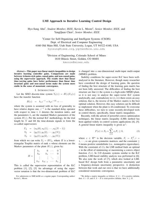
<strong>LMI</strong> <strong>Approach</strong> <strong>to</strong> <strong>Iterative</strong> <strong>Learning</strong> <strong>Control</strong> <strong>Design</strong><br />
Hyo-Sung Ahn † , Student Member, IEEE, Kevin L. Moore ‡ , Senior Member, IEEE, and<br />
YangQuan Chen † , Senior Member, IEEE<br />
† Center for Self-Organizing and Intelligent Systems (CSOIS)<br />
Dept. of Electrical and Computer Engineering<br />
4160 Old Main Hill, Utah State University, Logan, UT 84322-4160, USA<br />
hyosung@ieee.org, yqchen@ece.usu.edu<br />
Abstract— This paper uses linear matrix inequalities <strong>to</strong> design<br />
iterative learning controller gains. Comparisons are made<br />
between Arimo<strong>to</strong>-style gains, causal gains, and non-causal gains,<br />
using the supervec<strong>to</strong>r approach. The results show that linear<br />
time-varying gains have better performance than linear time<br />
invariant gains and non-causal terms make the system more<br />
stable in the sense of mono<strong>to</strong>nic convergence.<br />
I. INTRODUCTION<br />
Let the SISO discrete-time system Yk(z) = H(z)Uk(z)<br />
have the transfer function<br />
H(z) = h1z −1 + h2z −(2) + · · ·<br />
where the system is assumed with no loss of generality <strong>to</strong><br />
have relative degree one, z −1 is the standard delay opera<strong>to</strong>r<br />
with respect <strong>to</strong> time t, k denotes the iteration index, and<br />
the parameters hi are the standard Markov parameters of the<br />
system H(z). Per the normal ILC methodology, let the trial<br />
length be N and lift the time-domain signals <strong>to</strong> form the<br />
so-called supervec<strong>to</strong>rs:<br />
Uk = (uk(0), uk(1), · · · , uk(N − 1))<br />
Yk = (yk(1), yk(2), · · · , yk(N))<br />
Yd = (yd(1), yd(2), · · · , yd(N))<br />
from which we can write Yk = HUk, where H is a lowertriangular<br />
Toeplitz matrix of rank n whose elements are the<br />
Markov parameters of the plant H(z), given by:<br />
⎡<br />
⎢<br />
H = ⎢<br />
⎣<br />
‡ Division of Engineering, Colorado School of Mines<br />
1610 Illinois Street, Golden, CO 80401<br />
kmoore@mines.edu<br />
h1 0 · · · 0<br />
h2<br />
.<br />
h1<br />
.<br />
· · ·<br />
. ..<br />
0<br />
.<br />
hN hN−1 · · · h1<br />
This is called the supervec<strong>to</strong>r representation of the ILC<br />
problem [1], [2], [3] An advantage of using the supervec<strong>to</strong>r<br />
notation is that the two-dimensional problem of ILC<br />
For submission <strong>to</strong> SMCals/06 as a regular paper. Corresponding author:<br />
Kevin L. Moore<br />
⎤<br />
⎥<br />
⎦<br />
is changed in<strong>to</strong> a one-dimensional multi-input multi-output<br />
(MIMO) problem.<br />
Stability conditions for super-vec<strong>to</strong>r ILC have been wellanalyzed<br />
in the literature. However, though many researcher<br />
have considered the design of learning gains, the question<br />
of finding the best structure of the learning gain matrix has<br />
not been fully answered. The difficulties of finding the best<br />
structure are that (i) the system is a high-order MIMO plant,<br />
so it is not easy <strong>to</strong> analyze the super-vec<strong>to</strong>r ILC system<br />
analytically, and, contradic<strong>to</strong>ry <strong>to</strong> (i), (ii) there exists an easy<br />
solution, that is, the inverse of the Markov matrix is the best<br />
optimal solution. However, this easy solution can be difficult<br />
<strong>to</strong> implement when the plant is ill-conditioned. To overcome<br />
these difficulties, we turn <strong>to</strong> some recently-developed <strong>to</strong>ols<br />
in control theory, specifically, linear matrix inequalities.<br />
Recently, with the advent of powerful convex optimization<br />
techniques, the linear matrix inequality (<strong>LMI</strong>) method has<br />
been applied widely in control systems applications [4], [5].<br />
A general linear matrix inequality is given as1 :<br />
m<br />
F (x) ≡ F0 + xiFi ≥ 0, (1)<br />
i=1<br />
where x ∈ ℜm is the decision variable, Fi = F T i , i =<br />
1, · · · , m are given symmetric matrices, and the constraint ≥<br />
0 means positive semidefinite (i.e., nonnegative eigenvalues).<br />
With the constraint of (1), the <strong>LMI</strong> method finds an optimal<br />
x in the effort of minimizing or maximizing a convex object<br />
function J(x). In 2-D dynamic systems similar <strong>to</strong> the ILC<br />
problem, <strong>LMI</strong>-based stability analysis was performed in [6].<br />
We also note the work of [7], which also looked at <strong>LMI</strong>based<br />
ILC design both from a parametric uncertainty and<br />
a frequency-domain uncertainty perspective. A distinction<br />
between that work and our own is that we have additionally<br />
considered mono<strong>to</strong>nic convergence.<br />
1 We define a matrix inequality as follows: if A − B is positive definite,<br />
then A > B, and if A − B is semi-positive definite, then A ≥ B.
In this paper we show that the <strong>LMI</strong> method can be used<br />
<strong>to</strong> design the optimal ILC learning gain matrix. The paper<br />
is organized as follows. The super-vec<strong>to</strong>r ILC structure is<br />
analyzed in Section II Based on the analysis of Section II,<br />
<strong>LMI</strong> algorithms are designed in Section III and <strong>LMI</strong> test<br />
results are shown in Section IV. Conclusions are given in<br />
Section V.<br />
II. SUPER-VECTOR ILC ANALYSIS<br />
Consider the ILC update equation<br />
Uk+1 = Uk + ΓEk<br />
and the following definitions:<br />
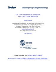
Definition 2.1: In the ILC learning gain matrix, a “band”<br />
is defined as sets of diagonals line as shown in Fig. 1.<br />
There are three different bands that we consider. “Arimo<strong>to</strong>type<br />
ILC gains or band” are considered a band of size one<br />
corresponding <strong>to</strong> the center diagonal of Γ, “causal ILC gains<br />
or bands” consist of diagonals that are below the center<br />
diagonal, and “non causal ILC gains or bands” consist of<br />
diagonals that are above the center diagonal. Causal and<br />
non-causal band sizes can vary according <strong>to</strong> the number of<br />
diagonals included. If the first causal and first non-causal<br />
diagonal are used, we call the band size 2. If the second<br />
causal and non-causal diagonals are used, the band size is 3.<br />
In this way we define the band size by the number causal<br />
and non-causal diagonals in the ILC gain matrix.<br />
Typical band<br />
Causal<br />
bands<br />
⎡γ<br />
⎢<br />
⎢<br />
γ<br />
⎢γ<br />
⎢<br />
⎢ M<br />
⎢<br />
⎣γ<br />
n<br />
11<br />
21<br />
31<br />
1<br />
γ<br />
γ<br />
γ<br />
γ<br />
Non- causal bands<br />
12<br />
22<br />
32<br />
M<br />
n2<br />
γ<br />
γ<br />
γ<br />
γ<br />
13<br />
23<br />
33<br />
M<br />
n3<br />
L<br />
L<br />
L<br />
O<br />
L<br />
γ 1n<br />
⎤<br />
γ<br />
⎥<br />
2n<br />
⎥<br />
γ ⎥ 3n<br />
⎥<br />
M ⎥<br />
γ ⎥<br />
nn ⎦<br />
Causal band<br />
size increases<br />
Non- causal band<br />
size increases<br />
Fig. 1. Band and band size in learning gain matrix<br />
Definition 2.2: We call Γ a linear time-invariant (LTI) ILC<br />
gain matrix if all the learning gain components in each<br />
diagonal are fixed as the same value. We call Γ a linear<br />
time-varying (LTV) ILC gain matrix if the learning gain<br />
components in each diagonal are different from each other.<br />
Definition 2.3: We define two stability concepts with respect<br />
<strong>to</strong> iteration: asymp<strong>to</strong>tic stability and mono<strong>to</strong>nic<br />
convergence. The system is asymp<strong>to</strong>tically stable if every<br />
finite initial state excites a bounded response, and the error<br />
ultimately approaches 0 as k → ∞. It is mono<strong>to</strong>nically<br />
convergent if ek+1 < ek, and ultimately approaches 0<br />
as k → ∞.<br />
For asymp<strong>to</strong>tic stability conditions, two concepts should be<br />
differentiated. When Arimo<strong>to</strong> or causal-only gains are used,<br />
the asymp<strong>to</strong>tic stability condition is defined as:<br />
|1 − γiih1| < 1, i = 1, · · · , n. (2)<br />
When non-causal gains are used in the ILC learning gain<br />
matrix the asymp<strong>to</strong>tic stability condition becomes:<br />
ρ(I − HΓ) < 1, (3)<br />
where ρ represents the spectral radius of (I − HΓ).<br />
On the other hand, mono<strong>to</strong>nic converegence is the same<br />
for all types of gain and requires:<br />
I − HΓi<br />
where · i represents the induced opera<strong>to</strong>r norm in the<br />
<strong>to</strong>pology of interest. In this paper we will consider the<br />
standard l1 and l∞ norm <strong>to</strong>pologies.<br />
In the following analysis, we consider four different cases:<br />
1) Arimo<strong>to</strong> gains with causal LTI gains<br />
2) Arimo<strong>to</strong> gains with causal LTV gains<br />
3) Arimo<strong>to</strong> gains with both causal and non-causal LTI<br />
gains<br />
4) Arimo<strong>to</strong> gains with causal and non-causal LTV gains<br />
First, we note the following observations, presented without<br />
proof:<br />
Lemma 2.1: In Case 1, the minimum of I − HΓ1 and<br />
I − HΓ∞ occurs if and only if Γ is exactly equal <strong>to</strong> the<br />
inverse of H.<br />
Lemma 2.2: In Case 2, Case 3 and Case 4, the minimum<br />
of I − HΓ1 and the minimum of I − HΓ∞ are zeros<br />
if and only if Γ is exactly equal <strong>to</strong> the inverse of H.<br />
Remark 2.1: From Lemma 2.1 and Lemma 2.2, we conclude<br />
that the best structure of Γ is the inverse of H. This is a<br />
necessary and sufficient condition. So, if the structure of the<br />
learning gain matrix is not fixed apriori, it is expected that<br />
the optimal Γ of the super-vec<strong>to</strong>r ILC would be the inverse of<br />
H. However, in super-vec<strong>to</strong>r ILC, it is unrealistic <strong>to</strong> assume<br />
that we know all Markov parameters exactly. Moreover, it is<br />
not advisable <strong>to</strong> use the inverse of H as the ILC learning gain<br />
matrix, because it is expensive <strong>to</strong> implement the inverse of<br />
H in the control loop when H is ill-conditioned. Therefore,<br />
we wish <strong>to</strong> use the <strong>LMI</strong> technique when the ILC gain has a<br />
fixed structure.<br />
Now, we analyze the learning gain matrix with a fixed<br />
band size. First, we compare LTI and LTV cases. We use<br />
following definitions:<br />
Definition 2.4: An LTI learning gain matrix with fixed<br />
band size is denoted as ΓLT I, and an LTV learning gain<br />
matrix with the same band size as ΓLT I is denoted as ΓLT V .<br />
Definition 2.5: When Γ is fixed as ΓLT I, the minimum of<br />
I − HΓLT I is denoted by J ∗ I ; and when Γ is fixed as<br />
ΓLT V , the minimum of I − HΓLT V is denoted by J ∗ V .
Then, using Definition 2.4 and Definition 2.5, we have<br />
following theorem, also stated without proof, from the fact<br />
that ΓLT I ⊂ ΓLT V .<br />
Theorem 2.1: If the same band size ILC gain matrices are<br />
used in ΓLT I and ΓLT V , the following inequality is satisfied:<br />
J ∗ V ≤ J ∗ I<br />
Remark 2.2: Theorem 2.1 relates the optimality between<br />
Case-1 and Case-2 and the optimality between Case-3 and<br />
Case-4. Also, from Theorem 2.1, the following corollary is<br />
immediate.<br />
Corollary 2.1: If the same band size is used in causal ILC<br />
and non-causal/causal ILC, then<br />
J ∗ N ≤ J ∗ C,<br />
where J ∗ N is the minimum value using causal, Arimo<strong>to</strong>, and<br />
non-causal learning gains; and J ∗ C is the minimum value<br />
using only causal and Arimo<strong>to</strong> gains.<br />
In summary, from Lemma 2.1 and Lemma 2.2, we conclude<br />
that the best gain matrix is just the inverse of H with<br />
respect <strong>to</strong> convergence in the l1 and l∞ norms. When the<br />
band size is fixed, we conclude that LTV is better than LTI<br />
from Theorem 2.1, and from Corollary 2.1 that including<br />
non-causal terms increases the optimality of the system.<br />
III. <strong>LMI</strong> DESIGN<br />
In this section, we show how <strong>to</strong> use <strong>LMI</strong> techniques for<br />
ILC design using several different fixed ILC gain matrix<br />
structures. Suppose we wish <strong>to</strong> satisfy the mono<strong>to</strong>nic convergence<br />
condition min[σ(I − HΓ)]. Now, because<br />
and because:<br />
σ[I − HΓ] ≡ λ([I − HΓ][I − HΓ] T ).<br />
λ([I − HΓ][I − HΓ] T ) ≤ [I − HΓ][I − HΓ] T <br />
then by minimizing [I − HΓ][I − HΓ] T , we can limit<br />
the upper bound of σ(I − HΓ). Because<br />
min( [I − HΓ][I − HΓ] T )<br />
is a typical matrix inequality problem, the ILC design problem<br />
can thus be solved by an <strong>LMI</strong>. We consider three cases:<br />
1. <strong>LMI</strong> − 1: Not-fixed learning gain matrix<br />
In <strong>LMI</strong> − 1, we do not fix the gain matrix structure, and<br />
the <strong>LMI</strong> algorithm finds the best structure by minimizing<br />
I − HΓ using Γ. A typical <strong>LMI</strong> is designed as<br />
subject <strong>to</strong><br />
max{−x 2 1}<br />
x 2 1In×n > [I − HΓ][I − HΓ] T . (4)<br />
However, (4) is a quadratic form, so we change (4) <strong>to</strong> a linear<br />
inequality form given by<br />
<br />
x1In×n [I − HΓ]<br />
[I − HΓ] T <br />
> 0 (5)<br />
x1In×n<br />
The more simplified form is designed according <strong>to</strong><br />
−x2 <br />
0 In×n H<br />
1I2n×2n −<br />
+ Γ [ 0 In×n ]<br />
In×n 0 0<br />
<br />
0<br />
+ ΓT [ HT 0 ] < 0. (6)<br />
In×n<br />
Then x1 is an optimization scalar variable and Γ is an<br />
optimization matrix variable.<br />
2. <strong>LMI</strong> − 2: LTI ILC with fixed band size<br />
As shown in Fig. 2.2 in the next section, the <strong>LMI</strong> algorithm<br />
finds the inverse of H as the optimal gain. This is already<br />
an expected result from the analysis of Section II. So, in this<br />
case, a big band-size gain matrix is indispensable. However,<br />
as already commented, the big band-size gain matrix is not<br />
practical. Thus, we design using <strong>LMI</strong>s by forcing a fixed<br />
gain matrix structure as shown in Fig. 1. For convenience,<br />
we use following learning gain matrix notation:<br />
⎡<br />
⎢<br />
Γ = ⎢<br />
⎣<br />
γp γ1 N γ2 N · · · γ n−1<br />
N<br />
γ1 C γp γ1 N · · · γ n−2<br />
N<br />
γ2 C γ1 C γp · · · γ n−3<br />
N<br />
. ..<br />
.<br />
γ n−1<br />
C<br />
.<br />
γ n−2<br />
C<br />
.<br />
γ n−3<br />
C · · · γp<br />
.<br />
⎤<br />
⎥<br />
⎦ ,<br />
where subscripts C, p, and N mean causal, Arimo<strong>to</strong> (proportional<br />
terms), and non-causal gains, respectively. The <strong>to</strong>tal<br />
number of variables in the learning gain matrix is 2n − 1.<br />
As already explained, if only γp is used in Γ, the band size<br />
is 1; if γp, γ1 C , and γ1 N are used, the band size is 2, and<br />
in the same way, if γp, γ 1 C ,· · ·,γk C , and γ1 N ,· · ·,γk N<br />
are used,<br />
the band size is k + 1. To design a linear <strong>LMI</strong>, we change<br />
I − HΓ <strong>to</strong><br />
In×n − [γ n−1<br />
C<br />
Hn−1<br />
C + · · · + γ1 CH1 C + γpHp<br />
+ · · · + γn−1 ], (7)<br />
+γ 1 N H1 N<br />
N Hn−1<br />
N<br />
where Hk C , k = 1, · · · , n−1 are Markov matrices corresponding<br />
<strong>to</strong> causal gains; Hp is a Markov matrix corresponding<br />
<strong>to</strong> Arimo<strong>to</strong> gains; and Hk N , k = 1, · · · , n − 1 are Markov<br />
matrices corresponding <strong>to</strong> non-causal gains. For example,<br />
they are expressed as:<br />
H 1 ⎡<br />
0 0 0 · · ·<br />
⎤<br />
0<br />
⎢<br />
C = ⎢<br />
⎣<br />
h1<br />
h2<br />
.<br />
0<br />
h1<br />
.<br />
0<br />
0<br />
.<br />
· · ·<br />
· · ·<br />
. ..<br />
0 ⎥<br />
0 ⎥<br />
.<br />
⎦<br />
hn−1 hn−2 hn−3 · · · 0
H 1 ⎡<br />
0 h1 0 · · ·<br />
⎤<br />
0<br />
⎢ 0<br />
⎢<br />
N = ⎢ 0<br />
⎢<br />
⎣<br />
.<br />
h2<br />
h3<br />
.<br />
h1<br />
h2<br />
.<br />
· · ·<br />
· · ·<br />
. ..<br />
0 ⎥<br />
0 ⎥<br />
.<br />
⎦<br />
0 hn hn−1 · · · h2<br />
Then, (7) is linear with respect <strong>to</strong> the learning gains. So the<br />
<strong>LMI</strong> method can be applied <strong>to</strong> the above expression, which<br />
gives a way for <strong>LMI</strong>-based LTI ILC. Finally, we change (7)<br />
in<strong>to</strong> an <strong>LMI</strong> form given by<br />
−x 2 <br />
1I2n×2n −<br />
0 In×n<br />
0<br />
with<br />
In×n<br />
<br />
0n×n Hp<br />
M1 =<br />
0n×n 0n×n<br />
M2 =<br />
+<br />
0n×n H 1 C<br />
0n×n 0n×n<br />
0n×n H n−1<br />
C<br />
0n×n 0n×n<br />
M3 =<br />
+<br />
0n×n H 1 N<br />
0n×n 0n×n<br />
0n×n H n−1<br />
N<br />
0n×n 0n×n<br />
<br />
<br />
+ M1 + M2 + M3 < 0, (8)<br />
γp + γp<br />
<br />
γ 1 C + γ1 C<br />
<br />
γ n−1<br />
C<br />
+ γn−1<br />
C<br />
<br />
γ 1 N + γ1 N<br />
<br />
γ n−1<br />
N<br />
+ γn−1<br />
N<br />
0n×n 0n×n<br />
H T p<br />
0n×n<br />
0n×n 0n×n<br />
<br />
,<br />
<br />
+ · · ·<br />
<br />
,<br />
(H1 C )T 0n×n<br />
<br />
0n×n 0n×n<br />
(H n−1<br />
C )T 0n×n<br />
0n×n 0n×n<br />
<br />
+ · · ·<br />
<br />
,<br />
(H1 N )T 0n×n<br />
<br />
0n×n 0n×n<br />
(H n−1<br />
N )T 0n×n<br />
where M1 denotes Ariomo<strong>to</strong> gain components, M2 the causal<br />
gain components, and M3 the non-causal gain components.<br />
Markov matrices are calculated from the algorithms in Table<br />
I, with the proportional term Markov matrix Hp = H.<br />
Note the MATLAB substitution notation is used in algorithms<br />
of Table I <strong>to</strong> Table III.<br />
TABLE I<br />
ALGORITHMS FOR MARKOV MATRICES OF LTI ILC<br />
LTI ILC algorithm<br />
for j = 1 : 1 : n − 1<br />
H j<br />
C (:, 1 : n − j) = H(:, j + 1 : n)<br />
H j<br />
C (:, n − j + 1 : n) = 0<br />
H j<br />
N (:, j + 1 : n) = H(j, 1 : n − j)<br />
H j<br />
N (:, 1 : j) = 0<br />
end<br />
Note that the LTI ILC algorithm includes causal gains,<br />
non-causal gains, and Arimo<strong>to</strong> gains. Thus, we have more<br />
flexibility <strong>to</strong> find the better learning gain matrix (Theorem<br />
2.1).<br />
3. <strong>LMI</strong> − 3: LTV ILC with fixed band size<br />
In LTV ILC, we use following learning gain matrix<br />
notation: ⎡<br />
γ11 γ12 · · ·<br />
⎤<br />
γ1n<br />
⎢ γ21<br />
Γ = ⎢<br />
⎣<br />
.<br />
γ22<br />
.<br />
· · ·<br />
. ..<br />
γ2n ⎥<br />
.<br />
⎦ .<br />
γn1 γn2 · · · γnn<br />
Like LTI ILC case, the band size is a design parameter. With<br />
the expanded I − HΓ in Lemma 2.2, and using the same<br />
procedure as LTI ILC, an <strong>LMI</strong> is designed as<br />
−x 2 n n<br />
0 In×n<br />
1I2n×2n−<br />
+ [Huγij +γijHl] < 0,<br />
0<br />
where<br />
In×n<br />
<br />
0n×n Hij<br />
Hu =<br />
0n×n 0n×n<br />
j=1 i=1<br />
<br />
0n×n<br />
; Hl =<br />
H T ij<br />
0<br />
0n×n<br />
Note that Hij are Markov matrices corresponding <strong>to</strong> the gains<br />
γij. If the band size is fixed as m, the algorithms of Table II<br />
and Table III are used <strong>to</strong> make <strong>LMI</strong> constraints. Then, the<br />
final Σ1 in Table II and the final Σ2 in Table III are summed<br />
<strong>to</strong> make linear matrix inequality constraints according <strong>to</strong><br />
(note that initially Σ1 and Σ2 are zero):<br />
−x 2 <br />
0 In×n<br />
1I2n×2n −<br />
0<br />
In×n<br />
TABLE II<br />
<br />
+ <br />
1<br />
+ <br />
2<br />
<br />
.<br />
(9)<br />
< 0. (10)<br />
ALGORITHMS FOR <strong>LMI</strong> CONSTRAINTS OF LTV CAUSAL AND ARIMOTO<br />
LTV Causal and Arimo<strong>to</strong><br />
GAINS<br />
for i = 1 : 1 : m<br />
for j = 1 : 1 : i<br />
for k = 1 : 1 : n − j + 1<br />
l = k + j − 1<br />
γ ′ = γkl<br />
R(1 : n, 1 : n) = 0<br />
R(1 : n, l) = H(1 : n, k)<br />
0n×0 R<br />
Σ1 = Σ1 +<br />
end<br />
end<br />
end<br />
0n×n 0n×n<br />
<br />
γ ′ + γ ′<br />
<br />
0n×n 0n×n<br />
RT <br />
0n×n<br />
IV. SIMULATION ILLUSTRATION<br />
In this section, the optimal learning gain matrices for four<br />
different cases are designed based on Section III algorithms.<br />
We use the following unstable system:<br />
⎡<br />
−0.50<br />
xk+1 = ⎣ 1.00<br />
0.00<br />
2.04<br />
⎤ ⎡<br />
0.00<br />
−1.20 ⎦ xk + ⎣<br />
0.00 1.20 0.00<br />
1.0<br />
⎤<br />
0.0 ⎦ (11)<br />
0.0<br />
yk = [ 1.0 2.5 −1.5 ] xk, (12)
TABLE III<br />
ALGORITHMS FOR <strong>LMI</strong> CONSTRAINTS OF LTV NON-CAUSAL GAINS<br />
LTV Non-causal<br />
for i = 1 : 1 : m<br />
for j = 1 : 1 : i − 1<br />
for k = j + 1 : 1 : n<br />
l = k − j<br />
γ ′ = γkl<br />
R(1 : n, 1 : n) = 0<br />
R(1 : n, l) = H(1 : n, k)<br />
0n×0 R<br />
Σ2 = Σ2 +<br />
end<br />
end<br />
end<br />
0n×n 0n×n<br />
<br />
γ ′ + γ ′<br />
<br />
0n×n 0n×n<br />
RT <br />
0n×n<br />
which has poles at [ 1.02 + j0.62, 1.02 − j0.62, −0.50 ] and<br />
zeros at [ 0.45, −0.91 ]. For <strong>LMI</strong> solutions, the free online<br />
Matlab software SeDuMi and SeDuMiInt were used [8],<br />
[9].<br />
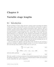
Test 1: Without using an <strong>LMI</strong> In this test, we just use<br />
Arimo<strong>to</strong>-type gains. From the plant dynamics we know that<br />
the first Markov parameter is h1 = CB = 1. So, with<br />
γp = 0.5 we know we will achieve asymp<strong>to</strong>tic stability.<br />
Fig. 2.1 shows the ILC result for the nominal system above.<br />
A sinusoidal reference signal was used. The figure shows the<br />
magnitude of the errors at each discrete time at the 2 nd , 3 rd ,<br />
4 th , and 5 th trials. Clearly the convergence is not mono<strong>to</strong>nic<br />
Test 2: Case-1 and Case-2 without fixing the band size<br />
Matching the analysis above from Section II, the <strong>LMI</strong><br />
solution determined that the inverse of the Markov parameters<br />
matrix was the optimal gain matrix. So, the l1-norm<br />
and l∞-norm are zero. Fig. 2.2 shows that the signal is<br />
mono<strong>to</strong>nically converging <strong>to</strong> the reference signal as iteration<br />
number increases.<br />
Test 3: Case-1 and Case-2 with fixed causal/Arimo<strong>to</strong> band<br />
size Fig. 2.3 shows the <strong>LMI</strong> test result with a learning gain<br />
matrix of causal/Arimo<strong>to</strong>, LTI with a fixed band size of<br />
3. The signal does not converge mono<strong>to</strong>nically. Fig. 2.4<br />
shows the <strong>LMI</strong> test result with learning gain matrix of<br />
causal/Arimo<strong>to</strong>, LTV with a fixed band size of 3. The LTV<br />
case shows much better performance than the LTI case, and<br />
the signal converges <strong>to</strong> the reference signal mono<strong>to</strong>nically.<br />
Test 4: Case-3 and Case-4 with fixed causal/Arimo<strong>to</strong>/noncausal<br />
band size Fig. 2.5 shows the <strong>LMI</strong> test result with a<br />
causal/Arimo<strong>to</strong>/non-causal band size of 3 and an LTI gain<br />
structure. Even though Fig. 2.5 shows much better performance<br />
than Fig. 2.3, it is still not mono<strong>to</strong>nically convergent.<br />
Still, we can conclude that LTV causal gains have better<br />
performance than LTI causal/noncausal gains. Fig. 2.6 shows<br />
the test result with a causal/Arimo<strong>to</strong>/non-causal band size of<br />
3 and an LTV gain structure. Fig. 2.6 shows that the signal<br />
converges <strong>to</strong> the reference signal mono<strong>to</strong>nically. From these<br />
figures, we conclude that causal/Arimo<strong>to</strong>/non-causal LTV has<br />
the best performance.<br />
V. CONCLUSION REMARKS<br />
In this paper we used <strong>LMI</strong> algorithms <strong>to</strong> find the best<br />
learning gain matrix structure in the super-vec<strong>to</strong>r ILC framework.<br />
From both analysis and <strong>LMI</strong> tests, we concluded that<br />
LTV is better than LTI, and non-causal terms can improve<br />
the mono<strong>to</strong>nic convergence of the system. In our future work<br />
we will consider two related questions: (i) how big should<br />
the band size be, a (ii) how can the <strong>LMI</strong>-based design be<br />
performed when rather than having knowledge of the matrix<br />
H we only have knowledge of upper and lower bounds on<br />
H (e.g., the case when H represents an interval plant).<br />
VI. REFERENCES<br />
[1] Kevin L. Moore, “Multi-loop control approach <strong>to</strong> designing<br />
iterative learning controllers,” in Proceedings of the<br />
37th IEEE Conference on Decision and <strong>Control</strong>, Tampa,<br />
Florida, USA, 1998, pp. 666–671.<br />
[2] J. J. Ha<strong>to</strong>nen D. H. Owens and K. L. Moore, “An<br />
algebraic approach <strong>to</strong> iterative learning control,” Int. J.<br />
<strong>Control</strong>, vol. 77, no. 1, pp. 45–54, 2004.<br />
[3] Kevin L. Moore, YangQuan Chen, and Vikas Bahl,<br />
“Mono<strong>to</strong>nically convergent iterative learning control for<br />
linear discrete-time systems,” in Submitted <strong>to</strong> Au<strong>to</strong>matica,<br />
pp. 1–16, July 2001.<br />
[4] Stephen Boyd, E. Feron, V. Balakrishnan, and L. El<br />
Ghaoui, “His<strong>to</strong>ry of linear matrix inequalities in control<br />
theory,” in Proc. American <strong>Control</strong> Conference, Baltimore,<br />
Maryland, USA., June 1994, AACC, pp. 31–34.<br />
[5] Didier Henrion, “Course on lmi optimization with<br />
applications in control,” Lecture Note, 2003.<br />
[6] K. Galkowski, J. Lam, E. Rogers, S. Xu, B. Sulikowski,<br />
W. Raszke, and D. H. Owens, “Lmi based stability<br />
anlaysis and robust controller design for discrete linear<br />
repetitive processes,” International Journal of Robust<br />
and Nonlinear <strong>Control</strong>, vol. 13, pp. 1195–1211, 2003.<br />
[7] Jian-Ming Xu, Ming-Xuan Sun, and Li Yu, “Lmi-based<br />
robust iterative learning controller design for discrete<br />
linear uncertain systems,” Journal of <strong>Control</strong> Theory<br />
and Applications, vol. 3, no. 2, pp. 259–265, 2005.<br />
[8] Jos F. Sturm, “Using sedumi 1.02, a matlab <strong>to</strong>olbox<br />
for optimization over symmectric cones,” Free On-line<br />
Software, Oc<strong>to</strong>ber 2001.<br />
[9] Dimitri Peaucelle, Didier Henrion, Yann Labit, and Krysten<br />
Taitz, “User’s guide for sedumi interface 1.04,” Free<br />
On-line Software, September 2002.
Errors<br />
Errors<br />
Errors<br />
30<br />
25<br />
20<br />
15<br />
10<br />
5<br />
2 nd trial<br />
3 rd trial<br />
4 th trial<br />
5 th trial<br />
0<br />
1 2 3 4 5 6 7 8 9 10<br />
Discrete Time<br />
0.9<br />
0.8<br />
0.7<br />
0.6<br />
0.5<br />
0.4<br />
0.3<br />
0.2<br />
0.1<br />
2 nd trial<br />
3 rd trial<br />
4 th trial<br />
5 th trial<br />
0<br />
1 2 3 4 5 6 7 8 9 10<br />
Discrete Time<br />
0.7<br />
0.6<br />
0.5<br />
0.4<br />
0.3<br />
0.2<br />
0.1<br />
2 nd trial<br />
3 rd trial<br />
4 th trial<br />
5 th trial<br />
0<br />
1 2 3 4 5 6 7 8 9 10<br />
Discrete Time<br />
Errors<br />
Errors<br />
Errors<br />
0.16<br />
0.14<br />
0.12<br />
0.1<br />
0.08<br />
0.06<br />
0.04<br />
0.02<br />
2 nd trial<br />
3 rd trial<br />
4 th trial<br />
5 th trial<br />
0<br />
1 2 3 4 5 6 7 8 9 10<br />
Discrete Time<br />
0.7<br />
0.6<br />
0.5<br />
0.4<br />
0.3<br />
0.2<br />
0.1<br />
2 nd trial<br />
3 rd trial<br />
4 th trial<br />
5 th trial<br />
0<br />
1 2 3 4 5 6 7 8 9 10<br />
Discrete Time<br />
0.7<br />
0.6<br />
0.5<br />
0.4<br />
0.3<br />
0.2<br />
0.1<br />
2 nd trial<br />
3 rd trial<br />
4 th trial<br />
5 th trial<br />
0<br />
1 2 3 4 5 6 7 8 9 10<br />
Discrete Time<br />
Fig. 2. ILC performances according <strong>to</strong> various band structures: Fig.2.1, upper-left: no <strong>LMI</strong>; Fig.2.2, upper-right: using H 1; Fig.2.3, middle-left: causal<br />
LTI with band size = 3; Fig.2.4, middle-right: causal LTV with band size = 3; Fig.2.5, bot<strong>to</strong>m-left: non-causal LTI with band size = 3; Fig.2.6, bot<strong>to</strong>m-right:<br />
non-causal LTV with band size = 3