LMI Approach to Iterative Learning Control Design - ResearchGate

H 1 ⎡
0 h1 0 · · ·
⎤
0
⎢ 0
⎢
N = ⎢ 0
⎢
⎣
.
h2
h3
.
h1
h2
.
· · ·
· · ·
. ..
0 ⎥
0 ⎥
.
⎦
0 hn hn−1 · · · h2
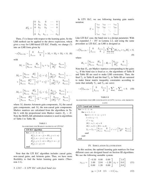
Then, (7) is linear with respect to the learning gains. So the
LMI method can be applied to the above expression, which
gives a way for LMI-based LTI ILC. Finally, we change (7)
into an LMI form given by
−x 2
1I2n×2n −
0 In×n
0
with
In×n
0n×n Hp
M1 =
0n×n 0n×n
M2 =
+
0n×n H 1 C
0n×n 0n×n
0n×n H n−1
C
0n×n 0n×n
M3 =
+
0n×n H 1 N
0n×n 0n×n
0n×n H n−1
N
0n×n 0n×n
+ M1 + M2 + M3 < 0, (8)
γp + γp
γ 1 C + γ1 C
γ n−1
C
+ γn−1
C
γ 1 N + γ1 N
γ n−1
N
+ γn−1
N
0n×n 0n×n
H T p
0n×n
0n×n 0n×n
,
+ · · ·
,
(H1 C )T 0n×n
0n×n 0n×n
(H n−1
C )T 0n×n
0n×n 0n×n
+ · · ·
,
(H1 N )T 0n×n
0n×n 0n×n
(H n−1
N )T 0n×n
where M1 denotes Ariomoto gain components, M2 the causal
gain components, and M3 the non-causal gain components.
Markov matrices are calculated from the algorithms in Table
I, with the proportional term Markov matrix Hp = H.
Note the MATLAB substitution notation is used in algorithms
of Table I to Table III.
TABLE I
ALGORITHMS FOR MARKOV MATRICES OF LTI ILC
LTI ILC algorithm
for j = 1 : 1 : n − 1
H j
C (:, 1 : n − j) = H(:, j + 1 : n)
H j
C (:, n − j + 1 : n) = 0
H j
N (:, j + 1 : n) = H(j, 1 : n − j)
H j
N (:, 1 : j) = 0
end
Note that the LTI ILC algorithm includes causal gains,
non-causal gains, and Arimoto gains. Thus, we have more
flexibility to find the better learning gain matrix (Theorem
2.1).
3. LMI − 3: LTV ILC with fixed band size
In LTV ILC, we use following learning gain matrix
notation: ⎡
γ11 γ12 · · ·
⎤
γ1n
⎢ γ21
Γ = ⎢
⎣
.
γ22
.
· · ·
. ..
γ2n ⎥
.
⎦ .
γn1 γn2 · · · γnn
Like LTI ILC case, the band size is a design parameter. With
the expanded I − HΓ in Lemma 2.2, and using the same
procedure as LTI ILC, an LMI is designed as
−x 2 n n
0 In×n
1I2n×2n−
+ [Huγij +γijHl] < 0,
0
where
In×n
0n×n Hij
Hu =
0n×n 0n×n
j=1 i=1
0n×n
; Hl =
H T ij
0
0n×n
Note that Hij are Markov matrices corresponding to the gains
γij. If the band size is fixed as m, the algorithms of Table II
and Table III are used to make LMI constraints. Then, the
final Σ1 in Table II and the final Σ2 in Table III are summed
to make linear matrix inequality constraints according to
(note that initially Σ1 and Σ2 are zero):
−x 2
0 In×n
1I2n×2n −
0
In×n
TABLE II
+
1
+
2
.
(9)
< 0. (10)
ALGORITHMS FOR LMI CONSTRAINTS OF LTV CAUSAL AND ARIMOTO
LTV Causal and Arimoto
GAINS
for i = 1 : 1 : m
for j = 1 : 1 : i
for k = 1 : 1 : n − j + 1
l = k + j − 1
γ ′ = γkl
R(1 : n, 1 : n) = 0
R(1 : n, l) = H(1 : n, k)
0n×0 R
Σ1 = Σ1 +
end
end
end
0n×n 0n×n
γ ′ + γ ′
0n×n 0n×n
RT
0n×n
IV. SIMULATION ILLUSTRATION
In this section, the optimal learning gain matrices for four
different cases are designed based on Section III algorithms.
We use the following unstable system:
⎡
−0.50
xk+1 = ⎣ 1.00
0.00
2.04
⎤ ⎡
0.00
−1.20 ⎦ xk + ⎣
0.00 1.20 0.00
1.0
⎤
0.0 ⎦ (11)
0.0
yk = [ 1.0 2.5 −1.5 ] xk, (12)