- Page 1 and 2: NASA Conference Publication 3352 <s
- Page 3 and 4: .Y NASA Conference Publication 3352
- Page 5 and 6: PREFACE Thisvolumecontainstheprocee
- Page 7 and 8: ORGANIZING COMMITTEE This workshop
- Page 9 and 10: CONTENTS Preface ..................
- Page 11 and 12: Large-Eddy Simulation of a High Rey
- Page 13 and 14: Problem 1 Benchmark Problems Catego
- Page 15 and 16: Problem 4 This is the same as Probl
- Page 17 and 18: , / circilar duct I incoming sound
- Page 19 and 20: Computational __ D
- Page 21 and 22: where ANALYTICAL SOLUTIONS OF THE C
- Page 23 and 24: The Greens function for (18)- (19)
- Page 25 and 26: where b = In2/w 2. Boundary conditi
- Page 27 and 28: SCATTERING OF SOUND BY A SPHERE: CA
- Page 29 and 30: where h O) (z) is the spherical Han
- Page 31 and 32: RADIATION OF SOUND FROM A POINT SOU
- Page 33 and 34: ef. 6. Theincident pressureemitted
- Page 35 and 36: 1 -g (Y3) lim .... - _ (X 3) - _ _
- Page 37 and 38: 7. , , . Martinez, R., "Liner Dissi
- Page 39 and 40: EXACT-SOLUTIONS FOR SOUND RADIATION
- Page 41 and 42: n=l Here R,.m is the conversion coe
- Page 43: where f_,(O) = (-i) ' J=(vm, )p24 (
- Page 47 and 48: As a approachesy, onereadilyobtains
- Page 49 and 50: It follows thenthat, as7/(0)approac
- Page 51: Ira(a) J . :::--::::::::_'.-.::, a=
- Page 54 and 55: n -3 -2 -1 0 +l 72 -6 -5 -4 -3 -2 -
- Page 57 and 58: Application of the Discontinuous Ga
- Page 59 and 60: eference1. In addition, the allowed
- Page 61 and 62: c_ = i. $/Igl, and fl = j-_/l_l. Ea
- Page 63 and 64: (a). Pressurecontour at t = 10. P 0
- Page 65 and 66: i 0.01 : " o.o - _;" .:y I -0.01 _
- Page 67 and 68: ...... r=5.5 --r=7.5 8e-06_ A /_ l
- Page 69 and 70: COMPUTATION OF ACOUSTIC SCATTERING
- Page 71 and 72: five-stage Runge-Kutta scheme (Hu e
- Page 73 and 74: processing.Theunit processingtimewa
- Page 75 and 76: lo ! 51- o' -1o 10 0 -10 I , •
- Page 77 and 78: 0 ] ' ' ' f i , , , -10 -5 0 5 10 1
- Page 79 and 80: 0. _5 i 5,0000E-6 O.O000EO -5.O000E
- Page 81 and 82: o 13 soLvT ON Acoustic S ,ERIN PROB
- Page 83 and 84: Gaussgrid, Xj+I/2 , mapped onto [0,
- Page 85 and 86: The coefficients,a x and aY determi
- Page 87 and 88: -4 -2 0 2 4 Figure 2: Subdomain dec
- Page 89 and 90: four around the cylinder. The PML e
- Page 91 and 92: Application of Dispersion-Relation-
- Page 93 and 94: where damping factor v = eAr × A9
- Page 95 and 96:
O x 10-l° 4, , , , , .... i 3.5 1_
- Page 97 and 98:
DEVELOPMENT OF COMPACT WAVE SOLVERS
- Page 99 and 100:
supportedthat C3N is long-time stab
- Page 101 and 102:
Figure 2 shows intersectionsof hori
- Page 103:
0.08 0.06 0.04 0.02 -0.02 -0.04 0 C
- Page 106 and 107:
OV 10p --+---=0 0t 7- 00 Op 1 c)(rU
- Page 108 and 109:
parallel to the radial direction, s
- Page 110 and 111:
¢-_ 4e--10 3e--10 2e--10 le--10 0.
- Page 112 and 113:
[3L- 0.06 0.04 0.02 0.00 --0.02 ...
- Page 114 and 115:
over ahalf-plane.Theequationsusedar
- Page 116 and 117:
At the computational boundaries, fl
- Page 118 and 119:
esolution of the grid causing the s
- Page 120 and 121:
0.08 q'- I ' "'I ..... T--F --[ I I
- Page 122 and 123:
"o_ 0.05 0.04 0.03 0.02 0.01 -0.01
- Page 124 and 125:
Forbothproblems(1& 2 of Category1),
- Page 126 and 127:
0 -3 -6 -9 -12 -15 -18 -21 -24 -27
- Page 128 and 129:
0.07 0.06 0.05 0.04 0.03 0.02 0.01
- Page 131 and 132:
•sy" _'J ApplicationAbsorb,n..oun
- Page 133 and 134:
First, the grid pointswill be overc
- Page 135 and 136:
2.3.1 Results of Problem 1 2.3 Nume
- Page 137 and 138:
Ov Op 0--t-+ Or = 0 (7.2) Op Ou 0;,
- Page 139 and 140:
To absorbthe out-goingwavesat thefa
- Page 141 and 142:
4.2 Inflow condition At the inflow,
- Page 143 and 144:
and u-velocity contours. In the vel
- Page 145 and 146:
mtel r BPouMLary Condition Figure 1
- Page 147 and 148:
0°0005 0.0004 0.0003 0.0002 0.0001
- Page 149 and 150:
5 0 -5 Figure 7a. 0 -5 Figure 7b. i
- Page 151 and 152:
008 006 0,04 i 0.02 O,., 0.0 13, .0
- Page 153 and 154:
i / Figure 13. Pressure contours at
- Page 155 and 156:
100 i0 -I 10 -z i0"3 10 .4 lO-s Fig
- Page 157 and 158:
100 i0 "] i0 "_ e_ i0 "s 10 -4 10 -
- Page 159 and 160:
4.0 3,0 2.5 2.0 0.0 4.0 _-._-,_ 3.0
- Page 161 and 162:
5.e-07 4.5e-07 4.e-07 3.5e-07 ¢_¢
- Page 163:
5.e-07 | 4.5e-07 I 4.e-07 [ _ 2.5e-
- Page 166 and 167:
1 + 3 + (a) (b) Figure 1" Basic sec
- Page 168 and 169:
Unfortunately the resulting schemem
- Page 170 and 171:
Figure 3: A typical (but rather coa
- Page 172 and 173:
! -10.0 -3.3 3.3 10.0 Figure 5: Pre
- Page 174 and 175:
0.07 0.06 0.05 0.04 0,03 0.02 0.01
- Page 176 and 177:
CONCLUSIONS _Te have presented a pr
- Page 178 and 179:
The methodis basedon a least-square
- Page 180 and 181:
For the linear wave problem of Cate
- Page 182 and 183:
FIG.1 PROBLEM 2 OF CATEGORY 1 - ACO
- Page 184 and 185:
0 0 0 0 0 0 0 0 ! (e'£'],)d 172 -4
- Page 186 and 187:
"Z3 c_ E < Q "13 ii i {3. E < Fig.
- Page 188 and 189:
200 -100 FIG. 7 TIME HISTORY OF AN
- Page 191 and 192:
ABSTRACT ADEQUATE BOUNDARY CONDITIO
- Page 193 and 194:
}Ve note that each v (k) is determi
- Page 195 and 196:
FORMULATION OF THE PROBLEM AND THE
- Page 197 and 198:
where APPENDfX We considerthe follo
- Page 199 and 200:
0.06 0.01 -0.04 0.06 0.01 -0.04 m w
- Page 201:
i 0.05 - -0.00 - \ 0.05 - -0.00 - -
- Page 204 and 205:
ditions. The formulation and implem
- Page 206 and 207:
J ! s J 18D 4D 5D Figure 1. <strong
- Page 208 and 209:
10 -10 rm 3.0 2.5 2.0 1.5 1.0 0.5 .
- Page 210 and 211:
3. CATEGORY 2, PROBLEM 2 The axysim
- Page 212 and 213:
off the axis. Such a change often r
- Page 214 and 215:
In the space" below, we will concen
- Page 216 and 217:
3.5. Numerical Results 1 I 1 Three
- Page 218 and 219:
p(x) 2.0 1.5 1.0 0.5 0.0 2.0 1.5 1,
- Page 220 and 221:
p(x) 1.5 1.0 0.5 0.0 1.5 1.0 0.5 0.
- Page 222 and 223:
For the case w " _s_, there are thr
- Page 224 and 225:
where E is an (M + 1) x 5 matrix an
- Page 226 and 227:
The v-velocity component in the out
- Page 228 and 229:
Figure 17 shows the calculated pres
- Page 230 and 231:
10-6 4.0 3.0 1.0 0.0 0.0 1.0 2.0 3.
- Page 233 and 234:
7'/ L/3
- Page 235 and 236:
w E W C w s S [.;sing this ceil-cen
- Page 237 and 238:
neighbors are involved. Both of the
- Page 239 and 240:
3e- 10 2.5e-10 ._ 2e-10 e-, • 1.5
- Page 241:
Future work involves the inclttsiot
- Page 244 and 245:
NONLINEAR, HYBRID CODE The hybrid d
- Page 246 and 247:
z agree better now although there a
- Page 248 and 249:
Figure 1: Snapshot of the acoustic
- Page 250 and 251:
-11 -12 -13 --% oT .9o -14 -15 Cat
- Page 253 and 254:
THREE-DIMENSIONAL CALCULATIONS OF A
- Page 255 and 256:
the IBM SP2. The computational doma
- Page 257 and 258:
intersects the center of the sphere
- Page 259 and 260:
ON COMPUTATIONS OF DUCT ACOUSTICS W
- Page 261 and 262:
It can be easily seen that duct aco
- Page 263 and 264:
the duct diameter D for problem 1 a
- Page 265 and 266:
To fix "this problem, a multi-domai
- Page 267 and 268:
60.0 , _ , , ,. _- f , 40.0 j 20.0
- Page 269:
0.004 [-- ' r .... , - , ," . ....
- Page 272 and 273:
w .................... 0..IJ'_l._ .
- Page 274 and 275:
{u} B= P 0 U M_v { M_p+w } ooP D= 0
- Page 276 and 277:
aseline case, as it employed a very
- Page 278 and 279:
the incoming wavesolution from the
- Page 280 and 281:
P(z) 1.0 Pressure Envelope ((o=7.2)
- Page 282 and 283:
v.rti_'al ¢li_tlllb;tl_('v. ;t11,1
- Page 284 and 285:
,l,>mairlOD. the,_4,_'r_ll_[ mt_'_L
- Page 286 and 287:
This is r,',',,g1_iz_',l a,,__zl ,q
- Page 288 and 289:
i ..J 2o i ¢.5 04 -2 0 fj,o_ DDD \
- Page 290 and 291:
2 8 ]or o 0,0 02 0.I 0.6 \ Circumfe
- Page 292 and 293:
Numerical Algorithm Equations (1) c
- Page 294 and 295:
The results are divided into differ
- Page 296 and 297:
0.012 0.01 0.008 0.006 0.004 0.002
- Page 298 and 299:
2 ... - -_ Patternrepeats I -- [ --
- Page 301 and 302:
-- o26 -7/ COMPUTATION OF SOUND GEN
- Page 303 and 304:
2.0 1.0i CI (Im.)o.o i ; -1.0 -2.0
- Page 305 and 306:
120 100 SPL, dB (re: 20 _Pa) 8O L
- Page 307:
REFERENCES 1. Lighthill, M. J., "On
- Page 310 and 311:
Perform numerical simulations to es
- Page 312 and 313:
[ RANS - Dirichlet B.C [ NNNNe , Pe
- Page 314 and 315:
.? _i, _ 80 .... 6O O0 02 04 0.6 0.
- Page 317 and 318:
A VISCOUS/ACOUSTIC SPLITTING TECHNI
- Page 319 and 320:
Ov' _" v o%' u'v' , OV v' OV Uv' Vu
- Page 321 and 322:
2 2 2 2 +L_ °_ _[_-_)J--T[_+d _) T
- Page 323 and 324:
corrector method was chosen. It is
- Page 325 and 326:
where # = p', u',v',p'. At the oute
- Page 327 and 328:
Finally, the latter portions of the
- Page 329 and 330:
p' o oo_ 9'3 t3 O3 75 7O 65 Nearfie
- Page 331 and 332:
LARGE-EDDY SIMULATION OF A HIGH REY
- Page 333 and 334:
In the implementation of the modeli
- Page 335 and 336:
to Cs = C 1/2 = 0.1. These LES gave
- Page 337 and 338:
a) c) ! • t r 2 i " i Figure 2. C
- Page 339 and 340:
t))
- Page 341 and 342:
A COMPARATIVE STUDY OF LOW DISPERSI
- Page 343 and 344:
Naturally, a left upwinded formula
- Page 345 and 346:
where F and G are flux vectors, and
- Page 347 and 348:
temporal integration of the semi-di
- Page 349 and 350:
vent reflected numerical waves from
- Page 351 and 352:
0.5 0.4 0.3 0.2 0.1 -0.1 0.6 0.4 0.
- Page 353 and 354:
13- Q- 0.2 0.15 0.1 0.050 [ -0.05 -
- Page 355 and 356:
1 e-06 9e-07 8e-07 7e-07 6e-07 5e-0
- Page 357 and 358:
133 cL cL 0.008 0.006 0.004 0.002 -
- Page 359 and 360:
0.0014 0.0012 0.001 0.0008 0.0006 P
- Page 361:
OVERVIEW OF COMPUTED RESULTS Christ
- Page 364 and 365:
10 -10 13.0 _i,i_ Illlllll, H _l,,l
- Page 366 and 367:
0.05 0.00 -0.05 0.05 0.00 -0.05 0.0
- Page 368 and 369:
0,05 0.00 -0.05 0.05 p(t) 0.00 -0.0
- Page 371 and 372:
SOLUTION COMPARISONS. CATEGORY 1: P
- Page 373 and 374:
_-12 8 Cat 2, Prob 1 " [_ Myers (BE
- Page 375 and 376:
p2=D(8) o.010 0.009 0.008 O.O07 0.0
- Page 377 and 378:
_:D(O) 0,12 0.11 0.10 0.09 0.08 0.0
- Page 379 and 380:
i° o. $ £ ,./ q 0.00 I i 1 1 0.20
- Page 381 and 382:
er .< o
- Page 383 and 384:
a- < (J O O ¢q o O O d J J o 0.00
- Page 385 and 386:
SOLUTION COMPARISONS: CATEGORY 4 Ja
- Page 387:
presenceof thewind tunnelwalls. The
- Page 390 and 391:
i == Slrul and Pylon Fan-OGV Pressu
- Page 392 and 393:
z >, O I.O O O O O (:3 O Some of no