Master Dissertation
Master Dissertation
Master Dissertation
You also want an ePaper? Increase the reach of your titles
YUMPU automatically turns print PDFs into web optimized ePapers that Google loves.
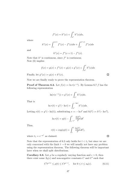
where<br />
and<br />
k ∗ (x) =<br />
f ∗ (x) = k ∗ x<br />
(x) +<br />
a∗ h ∗ (s)ds,<br />
x+1<br />
f<br />
x<br />
∗ (x) − f ∗ a∗ +1<br />
(s)ds +<br />
a∗ h ∗ (x) = f ∗ (x + 1) − f ∗ (x).<br />
Note that h∗ is continuous, since f ∗ is continuous.<br />
Now (6) implies<br />
f(x) = g(x) + f ∗ (x) = g(x) + g ∗ x<br />
(x) +<br />
a∗ Finally, let g ∗ (x) := g(x) + k ∗ (x).<br />
f ∗ (s)ds<br />
h ∗ (s)ds<br />
Now we are finally ready to prove the representation theorem.<br />
Proof of Theorem 6.2. Let f(x) := ln r(e−x ). By Lemma 6.7 f has the<br />
following representation<br />
That is<br />
ln(r(e −x )) = g ∗ x<br />
(x) +<br />
a∗ ln r(t) = g ∗ (− ln t) +<br />
− ln t<br />
a ∗<br />
h ∗ (s)ds.<br />
h ∗ (s)ds.<br />
Letting ν(t) := g ∗ (− ln(t)), substituting s := − ln t ′ and h(t ′ ) := h ∗ (− ln t ′ ),<br />
Thus,<br />
where t1 = e −a∗<br />
t<br />
ln r(t) = η(t) −<br />
e−a∗ h(t ′ )<br />
dt′<br />
t ′<br />
t1 h(t<br />
r(t) = exp(η(t) +<br />
t<br />
′ )<br />
t ′ dt′ ),<br />
as claimed.<br />
Note that the representation of 6.2 only holds for t < t1 but since we are<br />
only concerned with the limit t → 0 we will usually not have any problem<br />
using the representation theorem. The following theorem will be important<br />
later when we shall split distributions.<br />
Corollary 6.8. Let ρ be a regularly varying function and ɛ > 0, then<br />
there exist some S0(ɛ) and non-negative constants C and C ′ such that<br />
C ′ t ω+ɛ ≤ ρ(t) ≤ Ct ω−ɛ , for 0 ≤ t ≤ s0(ɛ). (6.11)<br />
47


