Equivalent temperature - Climate Science: Roger Pielke Sr.

Table 3
Annually-averaged 1982–1997 differences between TE and T trends
(and standard errors), with associated Z test statistic values testing
whether or not the trend differences are significantly different from
zero
Significance level ΔTE−ΔT (°C/decade) Z (ΔTE−ΔT)
All trends 0.021±0.004 4.88
N90% 1.068±0.190 5.62
N95% 1.475±0.289 5.10
N99% 1.910±0.582 3.28
Trend difference significance N90% if |Z|N1.65, significance N95% if |
Z|N1.96, and significance N99% if |Z|N2.58). Computations are done
for all individual trends and individual trends that are significant at or
above the 90%, 95%, and 99% significance levels. Each station is
weighted equally in each mean computation.
United States (Fig. 1) that are included in the International
Surface Weather Observations (ISWO) dataset, developed
at the National Climatic Data Center in Asheville,
North Carolina (NCDC, 1998). The ISWO dataset covers
the years 1982–1997, has undergone extensive quality
control, and consists of observations taken every 3 h.
Despite its short time span, the ISWO dataset is one of the
only near-surface air temperature datasets which also has
pressure and humidity observations, both of which are
needed to calculate T E. In addition, this time span is
adequate for investigating trend differences between Tand
T E rather than their actual trends. In this investigation, a
primary emphasis has been given to variations of temporal
trend differences between T and TE as a function of land
cover. Data from only the eastern U.S. were considered to
C.A. Davey et al. / Global and Planetary Change 54 (2006) 19–32
Table 4
Test statistic values for seasonally-averaged (winter, spring, summer,
fall) differences between TE and T trends, 1982–1997, for all
individual trends and individual trends that are significant at or
above the 90%, 95%, and 99% significance levels
Season All trends N90% N95% N99%
Winter (JFM) 6.14 5.14 4.05 2.27
Spring (AMJ) 6.62 3.53 2.69 0.58
Summer (JAS) 7.24 4.70 6.67 7.74
Fall (OND) −7.09 −5.10 −4.08 −4.58
Annual 4.88 5.62 5.10 3.28
Annually-averaged values are shown for comparison. Significance
criteria are identical to those specified in Table 3.
minimize effects of topography and because land cover
data were readily available for surface sites in that region
(Vogelmann et al., 2001).
Daily means of near-surface air temperature (T), dew
point temperature (T d), station elevation (z), and sea level
pressure (p o) were computed for each ISWO station.
Monthly means were then computed from the daily data.
From the monthly mean value for po,anapproximationof
the actual monthly mean pressure was calculated at each
site, using the formula
p ¼ poe −z=h ; ð3Þ
where z represents the elevation of the surface observation
station and h is the scale height. Once p was obtained, the
monthly mean specific humidity (q) and the mean equivalent
temperature (TE) werecalculated(Davey, 2005).
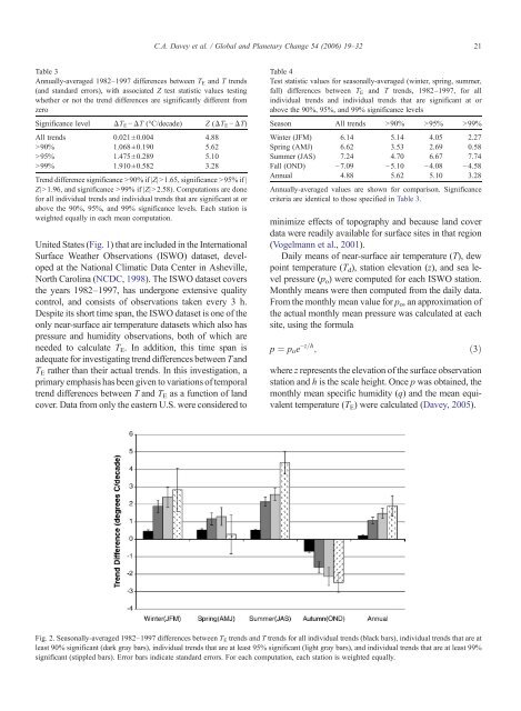
Fig. 2. Seasonally-averaged 1982–1997 differences between TE trends and T trends for all individual trends (black bars), individual trends that are at
least 90% significant (dark gray bars), individual trends that are at least 95% significant (light gray bars), and individual trends that are at least 99%
significant (stippled bars). Error bars indicate standard errors. For each computation, each station is weighted equally.
21