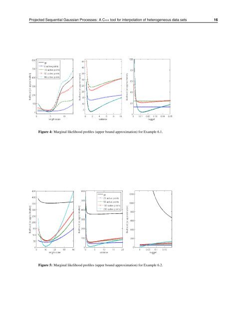
<strong>Projected</strong> <strong>Sequential</strong> <strong>Gaussian</strong> <strong>Processes</strong>: A <strong>C++</strong> <strong>tool</strong> <strong>for</strong> interpolation of heterogeneous data sets 16 Figure 4: Marginal likelihood profiles (upper bound approximation) <strong>for</strong> Example 6.1. Figure 5: Marginal likelihood profiles (upper bound approximation) <strong>for</strong> Example 6.2.
<strong>Projected</strong> <strong>Sequential</strong> <strong>Gaussian</strong> <strong>Processes</strong>: A <strong>C++</strong> <strong>tool</strong> <strong>for</strong> interpolation of heterogeneous data sets 17 6.3 Parameter estimation Figures 4 and 5 show the marginal likelihood profiles <strong>for</strong> the upper bound of the evidence (used to infer optimal hyper-parameters) <strong>for</strong> Example 6.1 and Example 6.2 respectively. These profiles show the objective function as a single hyper-parameter is varied while keeping the others fixed to their most likely values. The profiles are shown, from left to right, <strong>for</strong> the length scale (or range), the sill variance and the nugget variance. The objective function is evaluated <strong>for</strong> active sets of size 8 (diamonds), 16 (crosses), 32 (circles) and 64 (dots). For comparison, the full evidence, as given by a full <strong>Gaussian</strong> process (using the 64 observations) is plotted as a thick black line. For Example 6.1 (Figure 4), we observe in the region where the optimal hyper-parameters lie (corresponding to the minimum of the objective function) that the upper bound approximation to the true evidence (solid black line) provides a reasonable, but faster, substitute, as long as enough active points are retained. However, <strong>for</strong> low numbers of active points (8 or 16), the evidence with respect to the range and nugget terms is poorly approximated. In such cases, it is likely that the “optimal” range and nugget values will either be too large or too small depending on initialisation, resulting in unrealistic correlations and/or uncertainty in the posterior process. This highlights the importance of a retaining a large enough enough active set, the size of which will typically depend on the roughness of the underlying process, with respect to the typical sampling density. In the case of complex observation noise (Example 6.2, Figure 5), we can see that the profiles of the <strong>Gaussian</strong> process (GP) evidence and the psgp upper bound are very dissimilar, due to the different likelihood models used. The evidence <strong>for</strong> the GP reflects the inappropriate likelihood model by showing little confidence in the data (high optimal nugget value - not shown on the right hand plot due to a scaling issue) and difficulty in choosing an optimal set of parameters (flat profiles <strong>for</strong> the length scale and variance). Profiles <strong>for</strong> the psgp show much steeper minima <strong>for</strong> the range and variance, while keeping the nugget term very small (high confidence in the data). Again, this confirms that using a complex likelihood model is critical <strong>for</strong> extracting maximum in<strong>for</strong>mation from indirect observations or observations with non-<strong>Gaussian</strong> noise. 6.4 Application to spatial interpolation The third example shows an application of the psgp method to the interpolation of spatial observations. The dataset is taken from the INTAMAP case studies 8 . It consists of 2834 spatial measurements of gamma dose rate from the EURDEP monitoring network (Stöhlker et al., 2009). 566 observations are kept aside <strong>for</strong> validation and a psgp is fitted to the remaining ones in order to infer rates in regions where no data is available The psgp configuration used on that example includes the following settings: • the covariance function chosen is a mixture of a Matern 5/2, white noise and bias covariance functions. We also look at replacing the Matern 5/2 term with an Exponential covariance function to illustrate the flexibility of the model, • the size of the active set is limited to 400 active points, • hyper-parameters are estimated with a direct approximation to the evidence (based on the active set only), • prediction is done over a uni<strong>for</strong>m grid covering the data. 8 http://www.intamap.org/sample\_data.php\#radiation