Projected Sequential Gaussian Processes: A C++ tool for ... - MUCM

Projected Sequential Gaussian Processes: A C++ tool for interpolation of heterogeneous data sets 4
tion with respect to the underlying latent process at a point. The observation yi = y(xi) can
be directly of the underlying latent spatial process (with noise), i.e. yi = f (xi) + εi where
h is the identity mapping, but typically the sensor model might describe the observation
process or more simply be a mechanism for representing sensor bias using a linear sensor
model such as yi = [ f (xi) + b] + εi. It is possible that each sensor has a unique sensor
model, however it is more common for groups of sensors to have similar sensor models.
Note it will often be the case that each sensor has its own estimate of uncertainty, for
example where the observation results arise from processing raw data as seen in Boersma
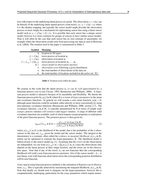
et al. (2004). The notation used in this paper is summarised in Table 2.
Symbol Meaning
x location in 2D space
fi = f (xi) latent process at location xi
yi = y(xi) observation at location xi
f = f 1:n = f (x1:n) latent process at locations x1,...,xn
h(·) sensor model or observation operator
ε observation error following a given distribution
n the total number of observations in the data set
m the total number of locations included in the active set, AS
Table 1: Notation used within the paper.
We assume in this work that the latent process is, or can be well approximated by, a
Gaussian process over x (see Cressie, 1993; Rasmussen and Williams, 2006). A Gaussian
process model is attractive because of its tractability and flexibility. We denote the
Gaussian process prior by p0( f |x,θ) where θ is a vector of hyper-parameters in the mean
and covariance functions. In general we will assume a zero mean function, µ(x) = 0,
although mean functions could be included, either directly or more conveniently by using
non-stationary covariance functions (Rasmussen and Williams, 2006, section 2.7). The
covariance function, c(x,x ′ ;θ), is typically parametrised by θ in terms of length scale
(range), process variance (sill variance) and nugget variance. A range of different valid
covariance functions are available, each of which imparts certain properties to realisations
of the prior Gaussian process. The posterior process is then given by:
ppost( f |y 1:n,x,θ,h) = p(y 1:n| f ,x,h)p0( f |x,θ)
p(y1:n| f ,x,h)p0( f |x,θ)d f
where p(y 1:n| f ,x,h) is the likelihood of the model, that is the probability of the n observations
in the data set, y 1:n, given the model and the sensor model. The integral in the
denominator is a constant, often called the evidence or marginal likelihood, p(y 1:n|x,θ),
which can be optimised to estimate the hyper-parameters, θ. The likelihood model is
linked closely to the sensor model eq. (1). Assuming that the errors on the observations
are independent, we can write p(y 1:n| f ,x) = ∏i pi(yi| f ,xi,hi) since the observations only
depend on the latent process at their single location, and the errors are in the observation
space. Note that if any of the errors, εi, are not Gaussian then the corresponding
likelihood will yield a non-Gaussian process posterior. Also if the sensor model – hi – is
non-linear, even with Gaussian observation errors the corresponding posterior distribution
will be non-Gaussian.
A key step in using Gaussian process methods is the estimation of θ given a set of observations,
y1:n. This is typically achieved by maximising the marginal likelihood, p(y 1:n|x,θ).
Note that ideally we should seek to integrate out the hyper-parameters, however this is
computationally challenging, particularly for the range parameters which require numer-
(2)