Projected Sequential Gaussian Processes: A C++ tool for ... - MUCM

More documents

Recommendations

Info

Projected Sequential Gaussian Processes: A C++ tool for interpolation of heterogeneous data sets 6 3 Interpolation for large data sets Techniques for treating large-scale spatial datasets can generally be organised into categories depending whether they utilise sparsely populated covariance matrices (Furrer et al., 2006), spectral methods (Fuentes, 2002) or low-rank covariance matrix approximations (Snelson and Ghahramani, 2006; Lawrence et al., 2003; Cressie and Johannesson, 2008). Each technique has associated advantages and disadvantages; here we consider low-rank covariance matrix approximations. A common technique for treating large-datasets is simply to sub-sample the dataset and use only a smaller number of observations during analysis. This is probably the most naïve low-rank covariance matrix approximation. All but the smaller subset of observations are discarded. Choosing the subset of observations that are to be retained can be complex. In Lawrence et al. (2003) the algorithm runs for a number of cycles sequentially inserting and removing observations determined by the magnitude of the reduction of uncertainty in the model. In this way a good subset of observations is chosen to represent the posterior process, although observations not within this subset will have no impact on the posterior, other than through the selection process. Csató and Opper (2002) present a similar approach, which is related to geostatistical theory in Cornford et al. (2005). Instead of discarding some observations, it is suggested that the effect of the discarded observations can be projected onto the low-rank covariance matrix in a sequential manner identifying the most informative observations in the process. It is shown how this can be done in such a way so as to minimise loss of information. Related to this is the technique of Snelson and Ghahramani (2006) where, instead of a sequential projection scheme, the entire dataset is projected on to a set of active points in a batch framework, a procedure that is complex. Cressie and Johannesson (2008) present an alternative where the Frobenius norm between the full and an approximate covariance matrices is minimised using a closed expression. The approach of Csató and Opper (2002), on which the psgp implementation is based, has a number of advantages. First, since it is a sequential algorithm (Opper, 1996), the complexity of the model, or the rank of the low-rank matrix can be determined during runtime. In scenarios where the complexity of the dataset is unknown a priori this is advantageous. Secondly, in a practical setting, it is not uncommon that observations arrive for processing sequential in time. Thirdly, by processing the data in a sequential fashion, non-Gaussian likelihoods, pi(yi| f ,xi,hi), can be used (Cornford et al., 2005). The projection step mentioned earlier is employed to project from a potentially non-Gaussian posterior distribution to the nearest Gaussian posterior distribution, again minimising the induced error in doing so. There are two ways in which the update coefficients, necessary for the projection, can be calculated: analytic methods requiring the first and second derivatives of the likelihood function with respect to the model parameters and by population Monte Carlo sampling (Cappé et al., 2004). The inclusion of this population Monte Carlo sampling algorithm is a novel feature of this implementation. The likelihood function for each observation can be described without having to calculate complex derivatives. Furthermore, our sampling based method enables sensor models, h[·] to be included, permitting data fusion. At present a basic XML parser is implemented which means that the psgp library can process sensor models described in MathML, as might be typical in a SensorML description in an Observations and Measurements document 2 part of the Sensor Web Enablement 3 suite of standards proposed by the Open Geospatial Consortium. 2 http://www.opengeospatial.org/standards/om 3 http://www.opengeospatial.org/ogc/markets-technologies/swe
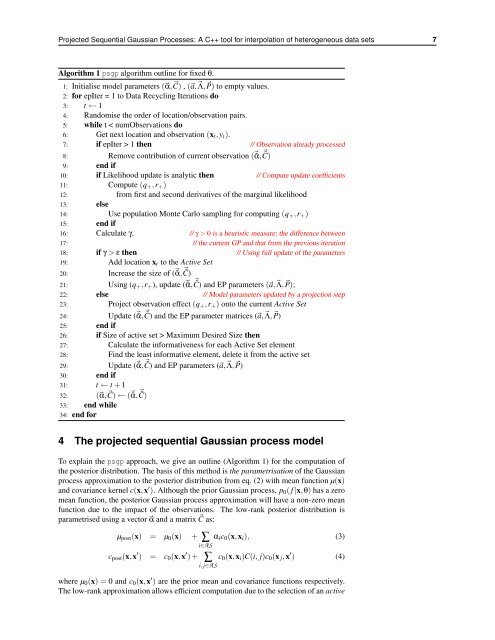
Projected Sequential Gaussian Processes: A C++ tool for interpolation of heterogeneous data sets 7 Algorithm 1 psgp algorithm outline for fixed θ. 1: Initialise model parameters (α,C) , (a,Λ,P) to empty values. 2: for epIter = 1 to Data Recycling Iterations do 3: t ← 1 4: Randomise the order of location/observation pairs. 5: while t < numObservations do 6: Get next location and observation (xt,yt). 7: if epIter > 1 then // Observation already processed 8: Remove contribution of current observation (˜α, ˜C) 9: end if 10: if Likelihood update is analytic then // Compute update coefficients 11: Compute (q+,r+) 12: from first and second derivatives of the marginal likelihood 13: else 14: Use population Monte Carlo sampling for computing (q+,r+) 15: end if 16: Calculate γ, // γ > 0 is a heuristic measure; the difference between 17: // the current GP and that from the previous iteration 18: if γ > ε then // Using full update of the parameters 19: Add location xt to the Active Set 20: Increase the size of (˜α, ˜C) 21: Using (q+,r+), update (˜α, ˜C) and EP parameters (a,Λ,P); 22: else // Model parameters updated by a projection step 23: Project observation effect (q+,r+) onto the current Active Set 24: Update (˜α, ˜C) and the EP parameter matrices (a,Λ,P) 25: end if 26: if Size of active set > Maximum Desired Size then 27: Calculate the informativeness for each Active Set element 28: Find the least informative element, delete it from the active set 29: Update (˜α, ˜C) and EP parameters (a,Λ,P) 30: end if 31: t ← t + 1 32: (α,C) ← (˜α, ˜C) 33: end while 34: end for 4 The projected sequential Gaussian process model To explain the psgp approach, we give an outline (Algorithm 1) for the computation of the posterior distribution. The basis of this method is the parametrisation of the Gaussian process approximation to the posterior distribution from eq. (2) with mean function µ(x) and covariance kernel c(x,x ′ ). Although the prior Gaussian process, p0( f |x,θ) has a zero mean function, the posterior Gaussian process approximation will have a non-zero mean function due to the impact of the observations. The low-rank posterior distribution is parametrised using a vector α and a matrix C as: µpost(x) = µ0(x) + ∑ αic0(x,xi), i∈AS (3) cpost(x,x ′ ) = c0(x,x ′ ) + ∑ i, j∈AS c0(x,xi)C(i, j)c0(x j,x ′ ) (4) where µ0(x) = 0 and c0(x,x ′ ) are the prior mean and covariance functions respectively. The low-rank approximation allows efficient computation due to the selection of an active
Page 1 and 2: Neural Computing Research Group Ast
Page 3 and 4: Projected Sequential Gaussian Proce
Page 5: Projected Sequential Gaussian Proce
Page 21: Projected Sequential Gaussian Proce

Projected Sequential Gaussian Processes: A C++ tool for ... - MUCM

You also want an ePaper? Increase the reach of your titles

Delete template?

Save as template?