Projected Sequential Gaussian Processes: A C++ tool for ... - MUCM

Projected Sequential Gaussian Processes: A C++ tool for interpolation of heterogeneous data sets 17
6.3 Parameter estimation
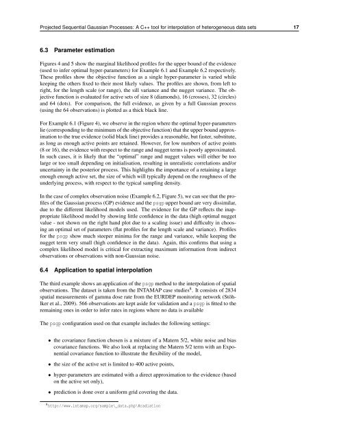
Figures 4 and 5 show the marginal likelihood profiles for the upper bound of the evidence
(used to infer optimal hyper-parameters) for Example 6.1 and Example 6.2 respectively.
These profiles show the objective function as a single hyper-parameter is varied while
keeping the others fixed to their most likely values. The profiles are shown, from left to
right, for the length scale (or range), the sill variance and the nugget variance. The objective
function is evaluated for active sets of size 8 (diamonds), 16 (crosses), 32 (circles)
and 64 (dots). For comparison, the full evidence, as given by a full Gaussian process
(using the 64 observations) is plotted as a thick black line.
For Example 6.1 (Figure 4), we observe in the region where the optimal hyper-parameters
lie (corresponding to the minimum of the objective function) that the upper bound approximation
to the true evidence (solid black line) provides a reasonable, but faster, substitute,
as long as enough active points are retained. However, for low numbers of active points
(8 or 16), the evidence with respect to the range and nugget terms is poorly approximated.
In such cases, it is likely that the “optimal” range and nugget values will either be too
large or too small depending on initialisation, resulting in unrealistic correlations and/or
uncertainty in the posterior process. This highlights the importance of a retaining a large
enough enough active set, the size of which will typically depend on the roughness of the
underlying process, with respect to the typical sampling density.
In the case of complex observation noise (Example 6.2, Figure 5), we can see that the profiles
of the Gaussian process (GP) evidence and the psgp upper bound are very dissimilar,
due to the different likelihood models used. The evidence for the GP reflects the inappropriate
likelihood model by showing little confidence in the data (high optimal nugget
value - not shown on the right hand plot due to a scaling issue) and difficulty in choosing
an optimal set of parameters (flat profiles for the length scale and variance). Profiles
for the psgp show much steeper minima for the range and variance, while keeping the
nugget term very small (high confidence in the data). Again, this confirms that using a
complex likelihood model is critical for extracting maximum information from indirect
observations or observations with non-Gaussian noise.
6.4 Application to spatial interpolation
The third example shows an application of the psgp method to the interpolation of spatial
observations. The dataset is taken from the INTAMAP case studies 8 . It consists of 2834
spatial measurements of gamma dose rate from the EURDEP monitoring network (Stöhlker
et al., 2009). 566 observations are kept aside for validation and a psgp is fitted to the
remaining ones in order to infer rates in regions where no data is available
The psgp configuration used on that example includes the following settings:
• the covariance function chosen is a mixture of a Matern 5/2, white noise and bias
covariance functions. We also look at replacing the Matern 5/2 term with an Exponential
covariance function to illustrate the flexibility of the model,
• the size of the active set is limited to 400 active points,
• hyper-parameters are estimated with a direct approximation to the evidence (based
on the active set only),
• prediction is done over a uniform grid covering the data.
8 http://www.intamap.org/sample\_data.php\#radiation