Projected Sequential Gaussian Processes: A C++ tool for ... - MUCM

More documents

Recommendations

Info

Projected Sequential Gaussian Processes: A C++ tool for interpolation of heterogeneous data sets 8 set AS = {x1,...,xm} of m locations where typically m ≪ n. Since psgp computation scales cubically with the size of the active set, m should be chosen as small as possible, however there is clearly a trade-off, which is discussed later. Computation of the parameters of the posterior parametrisation (the vector α and the matrix C) is a challenging task for a number of reasons. The parametrisation is an approximation that is based on the active set. Optimal active set locations depend on covariance function model parameters hence as these are re-estimated the active set must be reselected. The algorithm runs for a number of cycles and the processes of active set selection and covariance model parameter estimation are interleaved obtaining improved estimates during each cycle. Using the parametrisation from (3) and (4), the update rules are written as: αt+1 =αt + q+ st+1 Ct+1 = Ct + r+ st+1s T t+1 with st+1 = Ctct+1 +et+1 (5) where ct+1 = [c0(xt+1,x1),...,c0(xt+1,xt)] T is the prior covariance between the location being considered at iteration t + 1 and all current points in the active set. et+1 = [0,0,...,1] T is the t + 1-th unit vector that extends the size of αt+1 and Ct+1 by one. The consequence of the update rule is that: (1) all locations need to be processed since all of them contribute to the resulting mean and covariance functions, and (2) the contribution of each observation is retained in the posterior parametrisation. The benefits of the parametrisation and the sequential nature of the updates are two-fold. First, the update coefficients (q+ and r+) can be computed for a variety of user-defined likelihood models, pi(yi| f ,xi,hi), as shown in Section 4.1 and secondly, the update coefficients can be computed in a manner which does not require that the model complexity to be increased, as shown in Section 4.2. 4.1 Computing the update coefficients The update coefficients, q+ and r+, can be computed in two main ways. Essentially these update coefficients can be seen as computing the first two moments of the updated Gaussian approximation at xt+1, and thus require the evaluation of integrals. In Csató and Opper (2002) analytic formulations for q+ and r+ are given for Gaussian, Laplace and one sided exponential noise models. Within the psgp package at present only the Gaussian noise model is implemented analytically. In this paper we extend the updates to include a sampling based strategy, since the presence of a non-linear sensor model, h, will almost certainly make analytic updates impossible. The update step is iterated several times, within an inner loop to process all observations, and within an outer loop to recycle over data orderings, as shown in Algorithm 1. It is thus important that the computation of q+ and r+ is as efficient as possible. The sequential nature of the approximation means that the required integrals are low dimensional, and for scalar observations, one dimensional. Several methods might be envisaged, ranging from quadrature to Markov chain Monte Carlo methods. The selection of Population Monte Carlo (PMC) sampling (Cappé et al., 2004) was based on its simplicity and efficiency. PMC is a sequential importance sampling technique, where samples from one iteration are used to improve the importance sampling, or proposal, distribution at the subsequent steps in the algorithm. The technique is known to be efficient and we have found it to be stable too. The basic implementation is summarised in Algorithm 2. The main benefit of this approach is that one only needs to evaluate the sensor model forward to compute the likelihood of the observation p(yi| f ,xi,hi) and thus we can supply h as a MathML object to
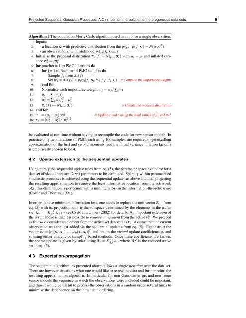
Projected Sequential Gaussian Processes: A C++ tool for interpolation of heterogeneous data sets 9 Algorithm 2 The population Monte Carlo algorithm used in psgp for a single observation. 1: Inputs: 2: - a location xi with predictive distribution from the psgp: p( fi|xi) = N(µi,σ 2 i ) 3: - an observation yi with likelihood pi(yi| fi,xi,hi) 4: Initialise the proposal distribution π∗( f ) = N(µ∗,σ 2 ∗) with µ∗ = µi and inflated variance σ 2 ∗ = sσ 2 i 5: for pmcIter = 1 to PMC Iterations do 6: for j = 1 to Number of PMC samples do 7: Sample f j from π∗( f ) 8: Set w j = π∗( f j) × pi(yi| f j,xi,hi) / p( f j|xi) // Compute the importance weights 9: end for 10: Normalise each importance weight w j = w j/∑k wk 11: µ∗ = ∑ j w j f j 12: σ2 ∗ = ∑ j w j f 2 j − µ2∗ 13: π∗( f ) ← N(µ∗,σ 2 ∗) 14: end for // Update the proposal distribution 15: q+ = (µ∗ − µi)/σ2 i // Update q and r using the final values of µ∗ and σ∗2 16: r+ = (σ 2 ∗ − σ 2 i )/(σ2 i )2 be evaluated at run-time without having to recompile the code for new sensor models. In practice only two iterations of PMC, each using 100 samples, are required to get excellent approximation of the first and second moments, and the initial variance inflation factor, s is empirically chosen to be 4. 4.2 Sparse extension to the sequential updates Using purely the sequential update rules from eq. (5), the parameter space explodes: for a dataset of size n there are O(n 2 ) parameters to be estimated. Sparsity within parametrised stochastic processes is achieved using the sequential updates as above and then projecting the resulting approximation to remove the least informative location from the active set, AS; this elimination is performed with a minimum loss in the information-theoretic sense (Cover and Thomas, 1991). In order to have minimum information loss, one needs to replace the unit vectoret+1 from eq. (5) with its projection πt+1 to the subspace determined by the elements in the active set: πt+1 = K −1 AS kt+1 – see Csató and Opper (2002) for details. An important extension of the result above is that it is possible to remove an element from the active set. We proceed as follows: consider an element from the active set denoted as x∗. Assume that the current observation was the last added via the sequential updates from eq. (5). Reconstruct the vectork∗ = [c0(x∗,x1),...,c0(x∗,xt)] T and obtain the virtual update coefficients q∗ and r∗ using either analytic or sampling based methods. Once these coefficients are known, the sparse update is given by substituting π∗ = K −1 AS k∗, where AS is the reduced active set in eq. (5). 4.3 Expectation-propagation The sequential algorithm, as presented above, allows a single iteration over the data-set. There are however situations when one would like to re-use the data and further refine the resulting approximation algorithm. In particular for non-Gaussian errors and non-linear sensor models the sequence in which the observations were included could be important, and thus it would be useful to process the observations in a random order several times to minimise the dependence on the initial data ordering.
Page 1 and 2: Neural Computing Research Group Ast
Page 3 and 4: Projected Sequential Gaussian Proce
Page 7: Projected Sequential Gaussian Proce
Page 21: Projected Sequential Gaussian Proce

Projected Sequential Gaussian Processes: A C++ tool for ... - MUCM

You also want an ePaper? Increase the reach of your titles

Delete template?

Save as template?