Projected Sequential Gaussian Processes: A C++ tool for ... - MUCM
Projected Sequential Gaussian Processes: A C++ tool for ... - MUCM
Projected Sequential Gaussian Processes: A C++ tool for ... - MUCM
You also want an ePaper? Increase the reach of your titles
YUMPU automatically turns print PDFs into web optimized ePapers that Google loves.
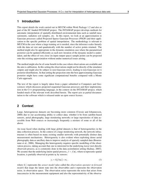
<strong>Projected</strong> <strong>Sequential</strong> <strong>Gaussian</strong> <strong>Processes</strong>: A <strong>C++</strong> <strong>tool</strong> <strong>for</strong> interpolation of heterogeneous data sets 3<br />
1 Introduction<br />
This report details the work carried out in <strong>MUCM</strong> within Work Package 1.2 and also as<br />
part of the EC funded INTAMAP project. The INTAMAP project develops methods <strong>for</strong><br />
automatic interpolation of spatially-distributed environmental data such as rainfall measurements,<br />
radiation soil samples, etc. In this report, we look at an approximation to<br />
<strong>Gaussian</strong> processes called <strong>Projected</strong> Sparse <strong>Gaussian</strong> <strong>Processes</strong> (PSGP) and their application<br />
to the specific problem of spatial interpolation. The methodology is relevant to<br />
<strong>MUCM</strong> in the case where a large training set is needed, since the inference scales linearly<br />
with the data set size and quadratically with the number of active points retained. The<br />
method might also be appropriate in the dynamic emulation case where the parametrised<br />
posterior can be updated efficiently as each new iteration of the dynamic model is undertaken,<br />
and the effect of very close (in input-output space) sample points can be projected<br />
onto the existing approximation without undue numerical issues arising.<br />
The method might also be of some benefit in the case where observations are available and<br />
the aim is calibration. In this setting the observations might not be directly of the simulator<br />
outputs and might also be subject to non-<strong>Gaussian</strong> errors, leading to non-<strong>Gaussian</strong> (or t)<br />
posterior distributions. In that setting the projection onto the best approximating <strong>Gaussian</strong><br />
posterior might have some significant computational benefits compared with a Monte<br />
Carlo approach.<br />
The text of the report is largely taken from a paper submitted to Computers and Geosciences<br />
which discusses projected sequential <strong>Gaussian</strong> processes and their implementation<br />
in the <strong>C++</strong> programming language, in the context on the INTAMAP project, which<br />
funded much of the relevant work described herein. The report acts as partial documentation<br />
to the software which is released under an open source licence.<br />
2 Context<br />
Large, heterogeneous datasets are becoming more common (Cressie and Johannesson,<br />
2008) due to our accelerating ability to collect data; whether it be from satellite-based<br />
sensors, aerial photography, large monitoring networks or large repositories of data accessible<br />
from Web sources or increasingly frequently a mixture of some or all of the<br />
above.<br />
An issue faced when dealing with large global datasets is that of heterogeneities in the<br />
data collection process. In the context of a large monitoring network, the network infrastructure<br />
is often based on many existing smaller networks with potentially distinct data<br />
measurement mechanisms. Heterogeneity is also evident when exploiting dense aerial<br />
photography data as ancillary data to improve analysis of sparsely sampled data (Bourennane<br />
et al., 2006). Managing this heterogeneity requires specific modelling of the observation<br />
process, taking account that one in interested in the underlying latent (not directly<br />
observed) process, as is commonly done in the data assimilation setting (Kalnay, 2003).<br />
We assume that the underlying latent spatial process, f = f (x), where x represents spatial<br />
location, is partially observed at points xi by sensors:<br />
yi = h[ f (xi)] + εi , (1)<br />
where h[·] represents the sensor model (also called the observation operator or <strong>for</strong>ward<br />
model) that maps the latent state into the observables and ε represents the observation<br />
noise, in observation space. The observation noise represents the noise that arises from<br />
inaccuracies in the measurement equipment and also the representativity of the observa-


