Projected Sequential Gaussian Processes: A C++ tool for ... - MUCM

Projected Sequential Gaussian Processes: A C++ tool for interpolation of heterogeneous data sets 19
The predictive mean and variances are shown in Figure 6 (centre and right plot, respectively)
along with the observation locations (left plot). Similar information is shown on
Figure 7, this time using an Exponential covariance function instead of the Matern 5/2.
In both cases, the mean process captures the main characteristics of the data although the
resulting mean field is a little too smooth for the Matern case in regions of high variability.
This is a problem often associated with stationary covariance functions, which assume the
spatial correlation of the data only depends on the distance between locations, not on the
locations themselves. Thus, the optimal set of hyper-parameters will try to accommodate
both the small scale and large scale patterns found in the data, favouring a good overall
fit at the expense of local accuracy. The addition to the framework of non-stationary covariance
functions and the use of more flexible mixtures of covariance functions could
help address this problem. The variance shows a rapid increase in uncertainty as we move
outside the observed area, which is expected given the local variability of the data.
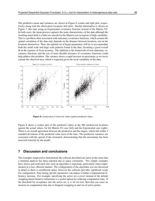
Figure 8: Scatter plot of observed values against predicted values.
Figure 8 shows a scatter plot of the predicted values at the 566 unobserved locations
against the actual values, for the Matern 5/2 case (left) and the Exponential case (right).
There is an overall agreement between the prediction and the targets, which fall within 2
standard deviations of the predicted value most of the time. The prediction variances are
consistent with the spread of the mismatch, demonstrating that the uncertainty has been
assessed correctly by the model.
7 Discussion and conclusions
The examples employed to demonstrate the software described are naïve in the sense that
a minimal analysis has been reported due to space constraints. Two simple examples
have shown and motivated why such an algorithm is important, particularly when implemented
in a fast, efficient manner. The configuration of the algorithm was not discussed
in detail as there is insufficient space, however the software provides significant scope
for configuration. Fine tuning specific parameters can induce a further computational efficiency
increase. For example, specifying the active set a priori instead of the default
swapping-based iterative refinement is a useful option for reducing computation time. If
the threshold for acceptance into the active set, γ, is set too low, then this can cause an
increase in computation time due to frequent swapping in and out of active points.