A particle-in-Burgers model: theory and numerics - Laboratoire de ...
A particle-in-Burgers model: theory and numerics - Laboratoire de ...
A particle-in-Burgers model: theory and numerics - Laboratoire de ...

You also want an ePaper? Increase the reach of your titles
YUMPU automatically turns print PDFs into web optimized ePapers that Google loves.
Mo<strong>de</strong>l <strong>and</strong> motivation Auxiliary steps Results h = 0: coupl<strong>in</strong>g h = 0: <strong>de</strong>f<strong>in</strong>ition, uniqueness h = 0: <strong>numerics</strong>, existence The coupled problem<br />
A <strong>particle</strong>-<strong>in</strong>-<strong>Burgers</strong> <strong>mo<strong>de</strong>l</strong>: <strong>theory</strong> <strong>and</strong><br />
<strong>numerics</strong><br />
B. Andreianov 1<br />
jo<strong>in</strong>t work with<br />
F. Lagoutière (Orsay), N. Segu<strong>in</strong> (Paris VI) <strong>and</strong> T. Takahashi (Nancy)<br />
1 <strong>Laboratoire</strong> <strong>de</strong> Mathématiques CNRS UMR6623<br />
Université <strong>de</strong> Franche-Comté<br />
Besançon, France<br />
September, 2011 — Ed<strong>in</strong>burgh<br />
Hyperbolic Conservation Laws<br />
<strong>and</strong> Related Analysis with Applications
Mo<strong>de</strong>l <strong>and</strong> motivation Auxiliary steps Results h = 0: coupl<strong>in</strong>g h = 0: <strong>de</strong>f<strong>in</strong>ition, uniqueness h = 0: <strong>numerics</strong>, existence The coupled problem<br />
Plan of the talk<br />
1 Mo<strong>de</strong>l <strong>and</strong> motivation<br />
2 Auxiliary steps<br />
3 Ma<strong>in</strong> Results<br />
4 The frozen <strong>particle</strong> case: coupl<strong>in</strong>g<br />
5 The frozen <strong>particle</strong> case: <strong>de</strong>f<strong>in</strong>ition, uniqueness<br />
6 The frozen <strong>particle</strong> case: <strong>numerics</strong> <strong>and</strong> existence<br />
7 The coupled problem
Mo<strong>de</strong>l <strong>and</strong> motivation Auxiliary steps Results h = 0: coupl<strong>in</strong>g h = 0: <strong>de</strong>f<strong>in</strong>ition, uniqueness h = 0: <strong>numerics</strong>, existence The coupled problem<br />
MODEL AND<br />
MOTIVATION
Mo<strong>de</strong>l <strong>and</strong> motivation Auxiliary steps Results h = 0: coupl<strong>in</strong>g h = 0: <strong>de</strong>f<strong>in</strong>ition, uniqueness h = 0: <strong>numerics</strong>, existence The coupled problem<br />
Mo<strong>de</strong>l <strong>and</strong> motivation...<br />
D’Alembert paradox : a solid immersed <strong>in</strong> an <strong>in</strong>viscid fluid is not<br />
submitted to any resultant force ; <strong>in</strong> other words, birds (<strong>and</strong> planes...)<br />
could not fly with a <strong>mo<strong>de</strong>l</strong> where viscosity is neglected ! Yet, <strong>in</strong>viscid<br />
(hyperbolic !) <strong>mo<strong>de</strong>l</strong>s are ok for some fluids...<br />
Answer 1 to the d’Alembert paradox: use viscous <strong>mo<strong>de</strong>l</strong>s of<br />
fluid-solid <strong>in</strong>teraction (see e.g. M. Hillairet , for a recent review).<br />
Answer 2 (when the Reynolds number is large): it is reasonable to<br />
neglect the viscous effects <strong>in</strong> the <strong>mo<strong>de</strong>l</strong> that governs the fluid ;<br />
but we have to conserve <strong>in</strong>formation from the vanish<strong>in</strong>g viscosity<br />
<strong>in</strong> a DRAG FORCE .<br />
The drag force takes the form of a source term which takes <strong>in</strong>to<br />
account the difference between the velocity of the fluid <strong>and</strong> the<br />
velocity of the solid.
Mo<strong>de</strong>l <strong>and</strong> motivation Auxiliary steps Results h = 0: coupl<strong>in</strong>g h = 0: <strong>de</strong>f<strong>in</strong>ition, uniqueness h = 0: <strong>numerics</strong>, existence The coupled problem<br />
...Mo<strong>de</strong>l <strong>and</strong> motivation...<br />
The 1D case : the Lagoutière-Segu<strong>in</strong>-Takahashi <strong>mo<strong>de</strong>l</strong> for the<br />
<strong>in</strong>teraction, via a drag force, of a po<strong>in</strong>t <strong>particle</strong> with a <strong>Burgers</strong> fluid<br />
writes<br />
∂tu +∂x(u 2 /2) = λ D(h ′ (t)−u) δ0(x − h(t)),<br />
here<br />
mh ′′ (t) = λ D(u(t, h(t)) − h ′ (t)).<br />
• u, the velocity of the fluid, is unknown<br />
• h, the position of the solid <strong>particle</strong>, is unknown<br />
(then h ′ <strong>and</strong> h ′′ respectively <strong>de</strong>note its velocity <strong>and</strong> acceleration);<br />
• the parameters are λ (the drag coefficient) <strong>and</strong> m (the mass of the<br />
solid <strong>particle</strong>); both are positive.<br />
• the function D which <strong>in</strong>tervenes <strong>in</strong> the drag force is an <strong>in</strong>creas<strong>in</strong>g<br />
odd function.<br />
Actually, we will suppose that<br />
either D(v) = v (the l<strong>in</strong>ear case)<br />
or D(v) = v|v| (the quadratic case).
Mo<strong>de</strong>l <strong>and</strong> motivation Auxiliary steps Results h = 0: coupl<strong>in</strong>g h = 0: <strong>de</strong>f<strong>in</strong>ition, uniqueness h = 0: <strong>numerics</strong>, existence The coupled problem<br />
AUXILIARY STEPS
Mo<strong>de</strong>l <strong>and</strong> motivation Auxiliary steps Results h = 0: coupl<strong>in</strong>g h = 0: <strong>de</strong>f<strong>in</strong>ition, uniqueness h = 0: <strong>numerics</strong>, existence The coupled problem<br />
Auxiliary steps to approach the full <strong>mo<strong>de</strong>l</strong>...<br />
Our study of the above coupled problem <strong>in</strong>clu<strong>de</strong>s two auxiliary steps,<br />
that are of <strong>in</strong>terest on their own. The first step is<br />
<br />
∂tu(t, x)+∂x(u 2 /2)(t, x) = −λ u(t, x) δ0(x), t > 0, x ∈ R,<br />
u(0, x) = u0(x), x ∈ R,<br />
i.e., the <strong>particle</strong> is <strong>de</strong>coupled from the fluid <strong>and</strong> fixed at zero.<br />
Difficulty 1 : the source term has to be carefully <strong>de</strong>f<strong>in</strong>ed. In<strong>de</strong>ed, u<br />
can be discont<strong>in</strong>uous (<strong>and</strong> <strong>in</strong> fact, typically u IS DISCONTINUOUS at<br />
the <strong>particle</strong> location ).<br />
To give an <strong>in</strong>terpretation of the source term, the LeRoux<br />
approximation was studied <strong>in</strong> <strong>de</strong>tail by Lagoutière, Segu<strong>in</strong>,<br />
Takahashi: δ0 = ∂xH (H: the Heavysi<strong>de</strong> function) is replaced by<br />
∂xHε, a smoothed version. This permits to un<strong>de</strong>rst<strong>and</strong> what goes on<br />
at the <strong>in</strong>terface.<br />
The second step is to take h(·) a given path, still <strong>de</strong>coupled from the<br />
fluid, <strong>and</strong> to solve the <strong>Burgers</strong> equation with s<strong>in</strong>gular source term<br />
located at x = h(t). We’ll see that as soon as the first step is well<br />
un<strong>de</strong>rstood, the second one is easy.
Mo<strong>de</strong>l <strong>and</strong> motivation Auxiliary steps Results h = 0: coupl<strong>in</strong>g h = 0: <strong>de</strong>f<strong>in</strong>ition, uniqueness h = 0: <strong>numerics</strong>, existence The coupled problem<br />
...Auxiliary steps to approach the full <strong>mo<strong>de</strong>l</strong><br />
Other way around, we should un<strong>de</strong>rst<strong>and</strong> how to evolve the <strong>particle</strong><br />
location given the fluid state at time t. Recall the equation (ODE) for<br />
the <strong>particle</strong>:<br />
mh ′′ (t) = λ (u(t, h(t)) − h ′ (t)).<br />
Recall that u(t,·) has a jump at x = h(t)...<br />
Difficulty 2 : un<strong>de</strong>rst<strong>and</strong> the equation <strong>in</strong> the Carathéodory sense ? In<br />
the Filippov sense ?? We will see that a nice mathematical <strong>and</strong><br />
physical <strong>in</strong>terpretation is possible:<br />
• the <strong>particle</strong> is driven by the lack of mass conservation <strong>in</strong> the<br />
equation for u ; or, equivalently, the total quantity of movement<br />
<br />
R u(t,·)+mh′ (t) is conserved.<br />
• the ODE for h can be written <strong>in</strong> a weak form that <strong>in</strong>volves the values<br />
of u(t,·) on R (which is more "robust")<br />
With these auxiliary steps well un<strong>de</strong>rstood, we can<br />
• th<strong>in</strong>k of the appropriate <strong>de</strong>f<strong>in</strong>ition of solution<br />
• use fixed-po<strong>in</strong>t arguments to guarantee existence<br />
• use time splitt<strong>in</strong>g algorithms (evolve the PDE <strong>and</strong> the ODE<br />
alternatively) for existence (constructive) <strong>and</strong> efficient <strong>numerics</strong>.
Mo<strong>de</strong>l <strong>and</strong> motivation Auxiliary steps Results h = 0: coupl<strong>in</strong>g h = 0: <strong>de</strong>f<strong>in</strong>ition, uniqueness h = 0: <strong>numerics</strong>, existence The coupled problem<br />
MAIN RESULTS
Mo<strong>de</strong>l <strong>and</strong> motivation Auxiliary steps Results h = 0: coupl<strong>in</strong>g h = 0: <strong>de</strong>f<strong>in</strong>ition, uniqueness h = 0: <strong>numerics</strong>, existence The coupled problem<br />
Ma<strong>in</strong> results: Auxiliary Problem 1 is well posed<br />
For the <strong>Burgers</strong>-with-Dirac-at-zero <strong>mo<strong>de</strong>l</strong> , we apply the mach<strong>in</strong>ery<br />
<strong>de</strong>veloped for conservation laws with discont<strong>in</strong>uous flux (adapted<br />
entropies, Baiti,Jenssen <strong>and</strong> Audusse,Perthame ; revisited <strong>and</strong><br />
generalized recently by BA., Karlsen, Risebro us<strong>in</strong>g the notion of<br />
admissibility germ ). The outcome is:<br />
– <strong>de</strong>f<strong>in</strong>ition(s) of entropy solutions<br />
– uniqueness, cont<strong>in</strong>uous <strong>de</strong>pen<strong>de</strong>nce (L 1 , L 1 loc<br />
<strong>de</strong>pen<strong>de</strong>nce) exactly as <strong>in</strong> the Kruzhkov <strong>theory</strong><br />
In addition, we f<strong>in</strong>d<br />
with doma<strong>in</strong> of<br />
– a priori L ∞ bounds <strong>and</strong> (more <strong>de</strong>licate) variation bounds<br />
– a strik<strong>in</strong>gly simple numerical method (monotone consistent f<strong>in</strong>ite<br />
volume scheme with a trick at the <strong>in</strong>terface )<br />
– convergence of the numerical scheme, existence .<br />
NB: the Riemann solver at the <strong>in</strong>terface was already <strong>de</strong>scribed by<br />
Lagoutière, Segu<strong>in</strong>, Takahashi , so a Godunov scheme could be<br />
constructed; but we seek to avoid us<strong>in</strong>g the Riemann solver because<br />
it is <strong>in</strong>tricate.
Mo<strong>de</strong>l <strong>and</strong> motivation Auxiliary steps Results h = 0: coupl<strong>in</strong>g h = 0: <strong>de</strong>f<strong>in</strong>ition, uniqueness h = 0: <strong>numerics</strong>, existence The coupled problem<br />
...Ma<strong>in</strong> results: : Auxiliary Problem 2 <strong>and</strong> the full problem<br />
Then for the <strong>Burgers</strong>-driven-by-<strong>particle</strong> <strong>mo<strong>de</strong>l</strong> (with x = h(t) GIVEN<br />
path of the <strong>particle</strong>) we <strong>de</strong>duce well-posedness rather easily.<br />
It is observed that the case of straight path, h(t) = Vt with V = const,<br />
reduces to the Dirac-at-zero <strong>mo<strong>de</strong>l</strong> by the simultaneous change of<br />
u − V <strong>in</strong>to u <strong>and</strong> of x − Vt <strong>in</strong>to x. Thus, noth<strong>in</strong>g new for h(t) = Vt.<br />
Then any (W 2,∞ ) path h(·) is approximated by piecewise aff<strong>in</strong>e paths;<br />
existence is established by passage to the limit. Uniqueness is<br />
straightforward from the <strong>de</strong>f<strong>in</strong>ition of solution.<br />
For the coupled <strong>mo<strong>de</strong>l</strong> with data u0 <strong>and</strong> h(0) = 0, h ′ (0) = v0, we get<br />
– existence, for L ∞ data u0<br />
– existence, uniqueness, cont<strong>in</strong>uous <strong>de</strong>pen<strong>de</strong>nce for BV solutions ,<br />
for BV data u0.<br />
We construct a time-explicit Glimm-type scheme where <strong>particle</strong><br />
position is updated via splitt<strong>in</strong>g; we get numerical results that agree<br />
with the physical phenomena that are expected for the <strong>mo<strong>de</strong>l</strong> .
Mo<strong>de</strong>l <strong>and</strong> motivation Auxiliary steps Results h = 0: coupl<strong>in</strong>g h = 0: <strong>de</strong>f<strong>in</strong>ition, uniqueness h = 0: <strong>numerics</strong>, existence The coupled problem<br />
FROZEN PARTICLE<br />
(DIRAC-AT-ZERO DRAG TERM):<br />
UNDERSTANDING THE COUPLING
Mo<strong>de</strong>l <strong>and</strong> motivation Auxiliary steps Results h = 0: coupl<strong>in</strong>g h = 0: <strong>de</strong>f<strong>in</strong>ition, uniqueness h = 0: <strong>numerics</strong>, existence The coupled problem<br />
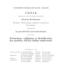
Frozen <strong>particle</strong>: un<strong>de</strong>rst<strong>and</strong><strong>in</strong>g the coupl<strong>in</strong>g...<br />
The admissibility at the <strong>in</strong>terface<br />
{x = 0} of the solution<br />
is governed by the germ Gλ<br />
(term<strong>in</strong>ology related to the one<br />
of BA, Karlsen, Risebro ):<br />
Def<strong>in</strong>ition<br />
The admissibility germ Gλ ⊂ R2 (or germ, for short) associated with<br />
the <strong>particle</strong>-at-zero problem is the union Gλ = G 1 λ ∪ G 2 λ ∪ G 3 λ , where<br />
= {(a, a−λ), a ∈ R}.<br />
G 1 λ<br />
G 2 λ<br />
= [0,λ]×[−λ, 0].<br />
(0, 0)<br />
G 3 λ = {(a, b) ∈ (R+ ×R− )\G 2 λ , −λ a+b λ}.<br />
NB: the partition of Gλ <strong>in</strong>to the three parts is dictated by the<br />
subsequent analysis, <strong>and</strong> by profiles study of LST .<br />
G 2 λ<br />
−λ<br />
u+<br />
λ<br />
G 1 λ<br />
G 3 λ<br />
u−
Mo<strong>de</strong>l <strong>and</strong> motivation Auxiliary steps Results h = 0: coupl<strong>in</strong>g h = 0: <strong>de</strong>f<strong>in</strong>ition, uniqueness h = 0: <strong>numerics</strong>, existence The coupled problem<br />
...Frozen <strong>particle</strong>: un<strong>de</strong>rst<strong>and</strong><strong>in</strong>g the coupl<strong>in</strong>g...<br />
Expla<strong>in</strong>ation : the <strong>Burgers</strong> equation with Dirac-at-zero drag term is<br />
equivalent to ∂tu +∂x(u 2 /2) = −λu∂xH.<br />
We <strong>in</strong>troduce Hε ∈ C 1 (R) a non-<strong>de</strong>creas<strong>in</strong>g function such that Hε(x) = H(x)<br />
when |x| ε. S<strong>in</strong>ce we are <strong>in</strong>terested <strong>in</strong> un<strong>de</strong>rst<strong>and</strong><strong>in</strong>g the behavior of the<br />
solution through the stationary <strong>in</strong>terface{x = 0}, we can study only<br />
stationary solutions. We then obta<strong>in</strong> the regularized equation for<br />
Uε(x) = u(t, x) <strong>in</strong> the strip −ε < x < ε:<br />
(U 2 ε/2) ′ (x)+λUε(x)∂xHε(x) = 0.<br />
Proposition (Lagoutière, Segu<strong>in</strong>, Takahashi ’08)<br />
In<strong>de</strong>pen<strong>de</strong>ntly from the choice of Hε, there exists a solution to the above<br />
ODE with Uε(−ε) = c− <strong>and</strong> Uε(+ε) = c+ if <strong>and</strong> only if (c−, c+) ∈ Gλ.<br />
The <strong>mo<strong>de</strong>l</strong>l<strong>in</strong>g assumption we make is the follow<strong>in</strong>g :<br />
the traces γ−u <strong>and</strong> γ+u at {x = 0} of a solution u of the <strong>Burgers</strong> equation on<br />
R + ×(R\{0}) are compatible if <strong>and</strong> only if there exists a solution to above<br />
ODE such that Uε(−ε) = γ−u, Uε(ε) = γ+u.<br />
Thus the germ Gλ is the set of couples(γ−u,γ+u) of possible traces at<br />
{x = 0} (for a.e. t > 0) of the admissible solutions.
Mo<strong>de</strong>l <strong>and</strong> motivation Auxiliary steps Results h = 0: coupl<strong>in</strong>g h = 0: <strong>de</strong>f<strong>in</strong>ition, uniqueness h = 0: <strong>numerics</strong>, existence The coupled problem<br />
...Frozen <strong>particle</strong>: un<strong>de</strong>rst<strong>and</strong><strong>in</strong>g the coupl<strong>in</strong>g...<br />
Now, the dissipativity properties of the <strong>in</strong>terface coupl<strong>in</strong>g are enco<strong>de</strong>d <strong>in</strong> the<br />
germ Gλ. In<strong>de</strong>ed, <strong>de</strong>f<strong>in</strong>e Ξ: R 2 ×R 2 ↦→ R by<br />
Ξ ± ((u−, u+),(v−, v+)) = Φ ± (u−, v−)−Φ ± (u+, v+)<br />
where Φ ± are the so-called semi-Kruzhkov entropy fluxes for <strong>Burgers</strong> eqn:<br />
Φ ± (u, v) = sgn ± (u − v)(u 2 − v 2 )/2.<br />
Splitt<strong>in</strong>g the germ Gλ <strong>in</strong>to three subsets, we have<br />
Proposition (dissipativity <strong>and</strong> maximality of Gλ)<br />
The follow<strong>in</strong>g properties hold:<br />
(i) (dissipativity) ∀(u−, u+),(v−, v+) ∈ Gλ,<br />
Ξ ± ((u−, u+),(v−, v+)) 0.<br />
(ii) (maximality + ...) If a pair (u−, u+) ∈ R 2 verifies:<br />
∀(v−, v+) ∈ G 1 λ ∪ G 2 λ Ξ((u−, u+),(v−, v+)) 0,<br />
then (u−, u+) ∈ Gλ.<br />
One can prove the proposition directly, by a tedious case study... but...
Mo<strong>de</strong>l <strong>and</strong> motivation Auxiliary steps Results h = 0: coupl<strong>in</strong>g h = 0: <strong>de</strong>f<strong>in</strong>ition, uniqueness h = 0: <strong>numerics</strong>, existence The coupled problem<br />
...Frozen <strong>particle</strong>: un<strong>de</strong>rst<strong>and</strong><strong>in</strong>g the coupl<strong>in</strong>g.<br />
A “better” (<strong>in</strong>direct) proof comes from the general <strong>theory</strong> from AKR .<br />
First, property (i) is actually equivalent to the “Kato <strong>in</strong>equality” (⇔<br />
L 1 -dissipativity)<br />
<br />
+ + <br />
− (u−v) ∂tϕ+Φ (u, v)∂xϕ 0 ∀ϕ ∈ D(Q), ϕ 0.<br />
R +<br />
R<br />
for the solutions<br />
u(t, x) := u−1l{x0}, v(t, x) := v−1l{x0}<br />
of our equation; <strong>and</strong> the Kato <strong>in</strong>equality comes by passage to the limit from<br />
the LeRoux approximation case :<br />
<br />
ε ε + ε ε + + ε ε<br />
λ(u −v ) (∂xHε)ϕ−(u −v ) ∂tϕ−Φ (u , v )∂xϕ 0.<br />
R +<br />
R<br />
Further, property (ii) means that “G 1 λ ∪ G 2 λ is a <strong>de</strong>f<strong>in</strong>ite germ of which Gλ is the<br />
unique maximal extension”. This follows (with some work) from the fact that<br />
Gλ is a complete germ (⇔ the germ allows to solve every Riemann problem).
Mo<strong>de</strong>l <strong>and</strong> motivation Auxiliary steps Results h = 0: coupl<strong>in</strong>g h = 0: <strong>de</strong>f<strong>in</strong>ition, uniqueness h = 0: <strong>numerics</strong>, existence The coupled problem<br />
FROZEN PARTICLE<br />
(DIRAC-AT-ZERO DRAG TERM):<br />
DEFINITION, UNIQUENESS
Mo<strong>de</strong>l <strong>and</strong> motivation Auxiliary steps Results h = 0: coupl<strong>in</strong>g h = 0: <strong>de</strong>f<strong>in</strong>ition, uniqueness h = 0: <strong>numerics</strong>, existence The coupled problem<br />
Frozen <strong>particle</strong>: <strong>de</strong>f<strong>in</strong>ition(s)...<br />
First, let us <strong>de</strong>scribe some elementary solutions of this problem:<br />
these are the stationary piecewise constant functions c:<br />
<br />
c− if x < 0,<br />
c(t, x) = c−1l {x0} = (c−, c+) ∈ Gλ.<br />
c+ if x > 0,<br />
They play the role of the constants <strong>in</strong> the st<strong>and</strong>ard Kruzhkov entropy<br />
formulation. With the i<strong>de</strong>a of adapted Kruzhkov entropies , we set up<br />
Def<strong>in</strong>ition (entropy solution)<br />
Let u0 ∈ L ∞ (R). A function u ∈ L ∞ (R + ×R) is said to be an entropy<br />
solution of the “<strong>particle</strong>-at-zero” problem if for all function c <strong>de</strong>f<strong>in</strong>ed<br />
above with (c−, c+) ∈ Gλ ,<br />
∀ϕ ∈ C ∞<br />
c (R + ×R), ϕ 0<br />
<br />
R +<br />
<br />
R<br />
[|u − c(x)| ∂tϕ+Φ(u, c(x)) ∂xϕ] dx dt<br />
<br />
+ |u0 − c(x)| ϕ(0, x) dx 0.<br />
R
Mo<strong>de</strong>l <strong>and</strong> motivation Auxiliary steps Results h = 0: coupl<strong>in</strong>g h = 0: <strong>de</strong>f<strong>in</strong>ition, uniqueness h = 0: <strong>numerics</strong>, existence The coupled problem<br />
...Frozen <strong>particle</strong>: <strong>de</strong>f<strong>in</strong>ition(s)...<br />
Let us provi<strong>de</strong> alternative characterizations of entropy solutions:<br />
Proposition (equivalent <strong>de</strong>f<strong>in</strong>itions)<br />
A function u ∈ L ∞ (R + ×R) is an entropy solution if <strong>and</strong> only if it satisfies any<br />
of the follow<strong>in</strong>g assertions:<br />
A. The function u verifies the adapted entropy <strong>in</strong>equalities with<br />
(c−, c+) ∈ G 1 λ ∪ G 2 λ.<br />
B. The function u verifies the Kruzhkov entropy <strong>in</strong>equalities for all<br />
nonnegative test function ϕ ∈ C ∞ c (R + ×R) such that ϕ|x=0 = 0,<br />
moreover,<br />
for a. e. t > 0 ((γ−u)(t), (γ+u)(t)) ∈ Gλ.<br />
D. There exists C = C(λ,u∞, c±) such that the function u verifies<br />
∀ϕ ∈ C ∞ c (R + <br />
×R), ϕ 0<br />
R +<br />
<br />
[|u−c(x)|∂tϕ+Φ(u, c(x))∂xϕ] dx dt<br />
R<br />
<br />
+ |u0 − c(x)| ϕ(0, x) dx −C(ϕ)dist<br />
R<br />
(c−, c+), Gλ)<br />
for all (c−, c+) ∈ R×R.
Mo<strong>de</strong>l <strong>and</strong> motivation Auxiliary steps Results h = 0: coupl<strong>in</strong>g h = 0: <strong>de</strong>f<strong>in</strong>ition, uniqueness h = 0: <strong>numerics</strong>, existence The coupled problem<br />
...Frozen <strong>particle</strong>: uniqueness, comparison, L 1 contraction.<br />
Theorem (L 1 contraction+comparison, analogous to Kruzhkov <strong>theory</strong>)<br />
Let u0 <strong>and</strong> v0 be two <strong>in</strong>itial data <strong>in</strong> L ∞ (R) <strong>and</strong> let u <strong>and</strong> v be the associated<br />
entropy solutions. Then for all R > 0,<br />
for a.e. t > 0<br />
R<br />
R<br />
(u − v) + (t, x) dx <br />
R+Lt<br />
(u0 − v0)<br />
−R−Lt<br />
+ (x) dx<br />
where L = max{u∞,v∞}. Consequently, if (u0 − v0) + ∈ L 1 (R), we have<br />
<br />
for a.e. t > 0 (u − v)<br />
R<br />
+ <br />
(t, x) dx (u0 − v0)<br />
R<br />
+ (x) dx.<br />
In particular, for all u0 ∈ L ∞ (R), there exists at most one solution <strong>and</strong> the map<br />
S(t) : u0 ↦→ u(t,·) on its doma<strong>in</strong> is an or<strong>de</strong>r-preserv<strong>in</strong>g L 1 contraction.<br />
The proof is straightforward us<strong>in</strong>g<br />
– the Kato <strong>in</strong>equality away from the <strong>in</strong>terface (st<strong>and</strong>ard Kruzhkov)<br />
– the characterization B. (“with traces” ) of entropy solutions<br />
– <strong>and</strong> the dissipativity of Gλ .
Mo<strong>de</strong>l <strong>and</strong> motivation Auxiliary steps Results h = 0: coupl<strong>in</strong>g h = 0: <strong>de</strong>f<strong>in</strong>ition, uniqueness h = 0: <strong>numerics</strong>, existence The coupled problem<br />
FROZEN PARTICLE<br />
(DIRAC-AT-ZERO DRAG TERM):<br />
NUMERICAL SCHEME AND EXISTENCE
Mo<strong>de</strong>l <strong>and</strong> motivation Auxiliary steps Results h = 0: coupl<strong>in</strong>g h = 0: <strong>de</strong>f<strong>in</strong>ition, uniqueness h = 0: <strong>numerics</strong>, existence The coupled problem<br />
Frozen <strong>particle</strong>: a f<strong>in</strong>ite volume scheme...<br />
We use a well-balanced f<strong>in</strong>ite volume scheme , preserv<strong>in</strong>g exactly<br />
(some of) the stationary sols u(t, x) := u−1l {x0}.<br />
Usual schemes are <strong>de</strong>term<strong>in</strong>ed by a numerical flux g(·,·) :<br />
– g locally Lipschitz;<br />
– g(u, u) = u2<br />
2 (consistency );<br />
– g(·, b) is ր, g(a,·) is ց (monotonicity ).<br />
We only modify g(·,·) at the <strong>in</strong>terface x = 0 (between x0 <strong>and</strong> x1):<br />
g −<br />
λ<br />
(a, b) = g(a, b + λ) <strong>and</strong> g+<br />
λ (a, b) = g( a − λ,b).<br />
I<strong>de</strong>a : g ±<br />
λ “only see” the G 1 λ part of the germ !<br />
Then the scheme writes<br />
∀i = 0, 1 u n+1<br />
i = u n i<br />
i = 0 : u n+1<br />
0 = un 0<br />
i = 1 : u n+1<br />
1<br />
Numerical solution:<br />
u∆(t, x) = <br />
n∈N<br />
− ∆t<br />
∆x (g(un i , un i+1 )−g(un i−1 , un i ));<br />
∆t − ∆x (g− λ (un 0 , un 1 )−g(un −1 , un 0 ));<br />
= un 1 − ∆t<br />
∆x (g(un 1, u n 2)−g +<br />
λ (un 0, u n 1)).<br />
<br />
i∈Z un i 1l (n∆t,(n+1)∆t)(t) 1l (xi−1/2,x i+1/2)(x).
Mo<strong>de</strong>l <strong>and</strong> motivation Auxiliary steps Results h = 0: coupl<strong>in</strong>g h = 0: <strong>de</strong>f<strong>in</strong>ition, uniqueness h = 0: <strong>numerics</strong>, existence The coupled problem<br />
Properties of the scheme...<br />
Un<strong>de</strong>r the CFL condition: 2M∆t ∆x, (M be<strong>in</strong>g the Lipschitz constant of<br />
the numerical flux g on the ad hoc <strong>in</strong>terval of values of (u n i )n,i, the scheme<br />
writes<br />
∀i ∈ Z u n+1<br />
i = Hi(u n i−1, u n i , u n i+1),<br />
where functions Hi are monotoneր <strong>in</strong> each of the three arguments.<br />
NB: s<strong>in</strong>ce · ↦→ ·±λ are ր functions, monotonicity OK also for i = 0, 1.<br />
Lemma (L ∞ bound — choice of M <strong>in</strong> the CFL condition)<br />
Un<strong>de</strong>r the CFL condition, the scheme satisfies for all n ∈ N, i ∈ Z<br />
m<strong>in</strong>{ess <strong>in</strong>f<br />
R − u0 −λ, ess <strong>in</strong>f<br />
R + u0} u n i max{ess sup<br />
Proposition (the scheme is (partially) well-balanced)<br />
R −<br />
u0, ess sup<br />
R +<br />
u0 +λ}.<br />
(i) The <strong>in</strong>itial datum v0(·) = c(·) = c−1l{x0},<br />
(c−, c+) ∈ G 1 λ, is exactly preserved <strong>in</strong> the evolution by the scheme .<br />
(ii) Let v∆ be the solution of the numerical scheme with<br />
the <strong>in</strong>itial datum v0(·) = c(·) = c−1l{x0},<br />
(c−, c+) ∈ G 2 λ. Then v∆ converge to c <strong>in</strong> L 1 loc(R + ×R) as ∆x → 0.
Mo<strong>de</strong>l <strong>and</strong> motivation Auxiliary steps Results h = 0: coupl<strong>in</strong>g h = 0: <strong>de</strong>f<strong>in</strong>ition, uniqueness h = 0: <strong>numerics</strong>, existence The coupled problem<br />
...Properties of the scheme...<br />
In what follows, we need a technical hypothesis (dissipativity at x = 0):<br />
(H) ∂a(∂ag(a, b)+∂bg(a, b)) 0, ∂b(∂ag(a, b)+∂bg(a, b)) 0;<br />
Lemma ( BVloc bound, Bürger, García, Karlsen, Towers )<br />
Let T > 0 <strong>and</strong> A > 0. Assume that u0 ∈ BV(R) <strong>and</strong> ∆x is small enough.<br />
Then, un<strong>de</strong>r the CFL condition <strong>and</strong> assumption (H), we have<br />
u∆(·,·)BV([0,T]×R\(−A,A)) 1<br />
Const(T,u0L ∞,u0BV(R),λ).<br />
A<br />
– estimate <strong>in</strong> BV(0, T; L 1 (R)) (i.e., time BV estimate <strong>in</strong> the mean ) from<br />
translation <strong>in</strong>variance + contraction (use Cr<strong>and</strong>all-Tartar lemma + (H))<br />
– mean-value theorem: for some r ∈ (0, A), u(·,±r)BV(0,T) const/A<br />
– look at our solution as solution to a Cauchy-Dirichlet problem<br />
with BV <strong>in</strong>itial <strong>and</strong> boundary data.<br />
Proposition (approximate Kato <strong>in</strong>equality)<br />
Let u∆, v∆ be solutions of the scheme. Let ϕ ∈ D([0, T)×R), ϕ 0. Then<br />
<br />
− (u∆−v∆) + ∂tϕ+Φ + (u∆, v∆)∂xϕ Rem(∆x,ϕ).<br />
R +<br />
R<br />
Arguments: monotonicity of the scheme, consistency , the BVloc <strong>in</strong> space<br />
bound
Mo<strong>de</strong>l <strong>and</strong> motivation Auxiliary steps Results h = 0: coupl<strong>in</strong>g h = 0: <strong>de</strong>f<strong>in</strong>ition, uniqueness h = 0: <strong>numerics</strong>, existence The coupled problem<br />
Convergence; existence of entropy solutions.<br />
Theorem (convergence of the scheme; existence of solutions)<br />
Assume u0 ∈ L ∞ (R). Then, un<strong>de</strong>r the CFL condition <strong>and</strong> assumption (H), the<br />
numerical scheme converges <strong>in</strong> L 1 loc(R + ×R) to the unique entropy solution to<br />
“<strong>Burgers</strong> with <strong>particle</strong>-at-zero” problem when ∆x tends to 0.<br />
In particular, the problem is well-posed , for L ∞ data <strong>and</strong> L 1 loc topology.<br />
Proof.<br />
• First assume that u0 ∈ BV(R).<br />
– BVloc bounds yield compactness: we get u an accumulation po<strong>in</strong>t of (u∆)∆ ;<br />
– well-balance property for (c−, c+) ∈ G 1 λ ∪ G 2 λ yields enough explicit<br />
stationary solutions v∆ to the scheme (at least, at the limit ∆x → 0);<br />
– us<strong>in</strong>g the approximate Kato <strong>in</strong>equalities on u∆ <strong>and</strong> the above special<br />
solutions v∆, at the limit we get Kato <strong>in</strong>equalities...<br />
but, these are precisely the adapted entropy <strong>in</strong>equalities !!<br />
– then u is (the unique) entropy solution (use caract. A. of entropy sols).<br />
• For the general case u0 ∈ L ∞ (R) , localize us<strong>in</strong>g f<strong>in</strong>ite speed of<br />
propagation; approximate u0 by BV(R)∩L 1 (R) functions(u n 0)n Use discrete<br />
L 1 contraction <strong>and</strong> the result of the BV case.
Mo<strong>de</strong>l <strong>and</strong> motivation Auxiliary steps Results h = 0: coupl<strong>in</strong>g h = 0: <strong>de</strong>f<strong>in</strong>ition, uniqueness h = 0: <strong>numerics</strong>, existence The coupled problem<br />
COUPLED PROBLEM
Mo<strong>de</strong>l <strong>and</strong> motivation Auxiliary steps Results h = 0: coupl<strong>in</strong>g h = 0: <strong>de</strong>f<strong>in</strong>ition, uniqueness h = 0: <strong>numerics</strong>, existence The coupled problem<br />
Case h = h(t): existence, uniqueness<br />
Theorem (well-posedness for mov<strong>in</strong>g but <strong>de</strong>coupled <strong>particle</strong>)<br />
Given h(·) a C 1 path, there exists a unique entropy solution to the <strong>Burgers</strong><br />
equation with s<strong>in</strong>gular drag term −λ(u − h ′ (t))δ0(x − h(t)); (localized) L 1<br />
contraction property holds.<br />
Def<strong>in</strong>ition :<br />
– the germ Gλ changes <strong>in</strong>to (h ′ (t), h ′ (t))+Gλ;<br />
– versions B. (“with traces”) <strong>and</strong> D. (“adapted entropy <strong>in</strong>equalities with<br />
rema<strong>in</strong><strong>de</strong>r term”) permit to <strong>de</strong>f<strong>in</strong>e entropy solutions.<br />
Arguments :<br />
– for uniqueness, comparison, L 1 contraction: same technique;<br />
– for existence: use characterization D. (it is stable by passage to the limit!) ;<br />
– approximate h(·) by a family (hn)n of piecewise aff<strong>in</strong>e paths<br />
– construction of solutions for “<strong>particle</strong> at hn” is straightforward: h ′ n be<strong>in</strong>g<br />
piecewise constant, one changes variables to reduce to the “drag<br />
force-at-zero” case. Procedure restarted at each time where h ′ n jumps.<br />
– because h ′ n → h ′ , the associated germs converge; thus we pass to the limit<br />
<strong>in</strong> characterization D..
Mo<strong>de</strong>l <strong>and</strong> motivation Auxiliary steps Results h = 0: coupl<strong>in</strong>g h = 0: <strong>de</strong>f<strong>in</strong>ition, uniqueness h = 0: <strong>numerics</strong>, existence The coupled problem<br />
Case h = h(t): cont<strong>in</strong>uous <strong>de</strong>pen<strong>de</strong>nce en h(·)<br />
Uniqueness proof for the coupled problem relies on a Gronwall <strong>in</strong>equality,<br />
which <strong>in</strong> turn relies on a Lipschitz <strong>de</strong>pen<strong>de</strong>nce estimate for the map<br />
h(·) ↦→ u(·,·) .<br />
Theorem (<strong>de</strong>pen<strong>de</strong>nce of u on the path h(·))<br />
Assume u, û are entropy solutions correspond<strong>in</strong>g to the <strong>particle</strong>s located at<br />
h(·), ˆ h(·), respectively, with h(0) = 0 = ˆ h(0) <strong>and</strong> same <strong>in</strong>itial datum u0.<br />
Assume û ∈ L ∞ (0, T; BV(R)). Then for a.e. t ∈ (0, T),<br />
t<br />
u(t,·)−û(t,·) L1 (R) C(u∞,û∞,ûBV,λ) |h<br />
0<br />
′ (s)− ˆ h ′ (s)| ds.<br />
Arguments:<br />
– change of variables y = x − h(t), resp. x − h ′ (t). Two eqns, both with<br />
s<strong>in</strong>gularity at zero, come out, with different fluxes of the k<strong>in</strong>d u ↦→ u2<br />
2 − h′ (t)u.<br />
– use the techniques of <strong>de</strong>pen<strong>de</strong>nce of entropy solutions on the flux function<br />
(BV regularity nee<strong>de</strong>d!): Kuznetsov, Bouchut-Perthame, Karlsen-Risebro... :<br />
the C 1 norm of the difference of the fluxes pops up, which yields |h ′ − ˆ h ′ |<br />
– use Lipschitz <strong>de</strong>pen<strong>de</strong>nce of the germ on h ′ to <strong>de</strong>scribe additional (small)<br />
“non-dissipation” term com<strong>in</strong>g from the <strong>in</strong>terface.
Mo<strong>de</strong>l <strong>and</strong> motivation Auxiliary steps Results h = 0: coupl<strong>in</strong>g h = 0: <strong>de</strong>f<strong>in</strong>ition, uniqueness h = 0: <strong>numerics</strong>, existence The coupled problem<br />
Case h = h(t): cont<strong>in</strong>uous <strong>de</strong>pen<strong>de</strong>nce en h(·), L ∞ <strong>and</strong> BV stability<br />
Proposition (BV estimate)<br />
The solution constructed for the h = 0 case obeys<br />
u(t,·)BV(R) ց for all t > 0<br />
(at t = 0 the variation may <strong>in</strong>crease by a const. <strong>de</strong>pend<strong>in</strong>g on u0∞,Gλ).<br />
The solution constructed for the fixed-h(·) case obeys the BV estimate<br />
u(t,·)BV(R) u0BV(R) + const(λ,u0∞)+2<br />
t<br />
0<br />
|h ′′ (s)| ds.<br />
Argument: (re)-construct solutions by wave-front track<strong>in</strong>g algorithm<br />
(Dafermos, Hol<strong>de</strong>n-Risebro, Bressan et al. ) (better control of <strong>in</strong>teractions).<br />
Lemma (L ∞ bounds)<br />
We get a uniform L ∞ bound on ad hoc sequences of h ′ (·) <strong>and</strong> u(·,·).<br />
To be precise: if we look at solutions to the coupled problem, we get<br />
max{u∞,h ′ ∞} max{u0∞,|h ′ (0)|}.<br />
For solutions appear<strong>in</strong>g <strong>in</strong> the fixed-po<strong>in</strong>t or splitt<strong>in</strong>g arguments, we get<br />
somewhat weaker bounds.
Mo<strong>de</strong>l <strong>and</strong> motivation Auxiliary steps Results h = 0: coupl<strong>in</strong>g h = 0: <strong>de</strong>f<strong>in</strong>ition, uniqueness h = 0: <strong>numerics</strong>, existence The coupled problem<br />
Case of u frozen: evolv<strong>in</strong>g h = h(·)<br />
Proposition (<strong>mo<strong>de</strong>l</strong>l<strong>in</strong>g/“traces” <strong>in</strong>terpretation of the ODE on h(·) )<br />
For every drag force, the ODE <strong>in</strong> the coupled problem writes<br />
mh ′′ <br />
(t) =<br />
−<br />
<br />
(u−) 2 /2−h ′ (t)u−<br />
<br />
(u+) 2 /2−h ′ (t)u+<br />
Notice that the right-h<strong>and</strong> si<strong>de</strong> above is expressed as the difference of the<br />
normal components of the 2D-field (u, u 2 /2) on the curve {x = h(t)} from<br />
the left <strong>and</strong> from the right . Comb<strong>in</strong><strong>in</strong>g this observation with the Green-Gauss<br />
formula, we get the follow<strong>in</strong>g weak formulation of the ODE:<br />
Lemma (second <strong>in</strong>terpretation of the ODE on h(·) )<br />
Let u be a weak solution of the PDE on {x = h(t)}; let h ∈ W 2,∞ (0, T). Then<br />
h(·) verifies the ODE if <strong>and</strong> only if for all ξ ∈ D([0, T)), for all ψ ∈ D(R) such<br />
that ψ ≡ 1 on the set {x ∈ R : ∃t ∈ [0, T] such that h(t) = x}, there holds<br />
T<br />
−m h<br />
0<br />
′ (t)ξ ′ (t)dt = mh ′ T <br />
(0)ξ(0)+ uψξt +<br />
0 R<br />
u2<br />
2 ξψx<br />
<br />
+ u0ψξ(0).<br />
R<br />
<br />
.
Mo<strong>de</strong>l <strong>and</strong> motivation Auxiliary steps Results h = 0: coupl<strong>in</strong>g h = 0: <strong>de</strong>f<strong>in</strong>ition, uniqueness h = 0: <strong>numerics</strong>, existence The coupled problem<br />
Coupled problem: existence, uniqueness of BV solutions / existence of<br />
L ∞ solutions<br />
The above <strong>in</strong>gredients can be used <strong>in</strong> several ways:<br />
– In a fixed-po<strong>in</strong>t argument h(·) ↦→ u(·,·) ↦→ h(·)<br />
(compactness: work <strong>in</strong> C 1 ([0, T]), exploit a W 2,∞ (0, T) bound on h(·) )<br />
– In a time splitt<strong>in</strong>g algorithm (alternatively evolv<strong>in</strong>g u <strong>and</strong> h on small time<br />
<strong>in</strong>tervals):<br />
· u updated from h us<strong>in</strong>g the <strong>theory</strong> of entropy solutions for h frozen;<br />
· h updated from u us<strong>in</strong>g the above weak formulation of the ODE.<br />
– In a numerical scheme (same time splitt<strong>in</strong>g + approximation <strong>in</strong> space of the<br />
conservation law); an <strong>in</strong>terest<strong>in</strong>g possibility is the r<strong>and</strong>om-choice algorithm<br />
(Glimm ), <strong>in</strong> or<strong>de</strong>r not to adapt the space mesh<strong>in</strong>g to the <strong>particle</strong> location.<br />
Theorem (Ma<strong>in</strong> result)<br />
For all BV datum u0 <strong>and</strong> given h(0), h ′ (0), there exists a unique entropy<br />
solution to the coupled problem.<br />
For all L ∞ datum u0 <strong>and</strong> given h(0), h ′ (0), there exists an entropy solution to<br />
the coupled problem.
Mo<strong>de</strong>l <strong>and</strong> motivation Auxiliary steps Results h = 0: coupl<strong>in</strong>g h = 0: <strong>de</strong>f<strong>in</strong>ition, uniqueness h = 0: <strong>numerics</strong>, existence The coupled problem<br />
Coupled problem: a well-balanced r<strong>and</strong>om-choice numerical scheme<br />
t<br />
t n+1<br />
t n<br />
x<br />
g0(u n In−1, u n In )<br />
u n+1<br />
In<br />
u n uIn n In<br />
ũ n+1<br />
In<br />
h n + v n ∆t<br />
h n + y<br />
gv n(un In ,ϕ− α(u n In+1))<br />
xIn−1/2 h n = xIn+1/2<br />
gv n(ϕ+ α(u n In ), un In+1)<br />
u n+1<br />
In+1<br />
u n In+1<br />
ũ n+1<br />
In+1<br />
g0(u n In , un In+1)<br />
h n+1<br />
xIn+3/2<br />
Figure: Representation of the algorithm based on the well-balanced scheme.
Mo<strong>de</strong>l <strong>and</strong> motivation Auxiliary steps Results h = 0: coupl<strong>in</strong>g h = 0: <strong>de</strong>f<strong>in</strong>ition, uniqueness h = 0: <strong>numerics</strong>, existence The coupled problem<br />
Numerics: draft<strong>in</strong>g-kiss<strong>in</strong>g-tumbl<strong>in</strong>g<br />
t<br />
5<br />
4.5<br />
4<br />
3.5<br />
3<br />
2.5<br />
2<br />
1.5<br />
1<br />
0.5<br />
Particle 1<br />
Particle 2<br />
0<br />
0 0.2 0.4 0.6 0.8 1<br />
x<br />
Figure: Trajectories of two <strong>particle</strong>s
Mo<strong>de</strong>l <strong>and</strong> motivation Auxiliary steps Results h = 0: coupl<strong>in</strong>g h = 0: <strong>de</strong>f<strong>in</strong>ition, uniqueness h = 0: <strong>numerics</strong>, existence The coupled problem<br />
Thx !!!<br />
THANK YOU !