Modeling spatial population scenarios
Modeling spatial population scenarios
Modeling spatial population scenarios

You also want an ePaper? Increase the reach of your titles
YUMPU automatically turns print PDFs into web optimized ePapers that Google loves.
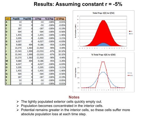
Results: Assuming constant r = -5%<br />
Cell Pop(0) Pop(50) ∆ Pop % ∆ Pop ∆ %Pop<br />
A 13 0 -13 -100% -0.01%<br />
B 53 0 -53 -100% -0.05%<br />
C 187 0 -187 -100% -0.19%<br />
D 564 0 -564 -100% -0.56%<br />
E 1,455 0 -1,455 -100% -1.46%<br />
F 3,205 0 -3,205 -100% -3.21%<br />
G 6,027 0 -6,027 -100% -6.03%<br />
H 9,680 494 -9,186 -95% -3.26%<br />
I 13,273 1,363 -11,910 -90% 4.44%<br />
J 15,543 1,990 -13,553 -87% 10.32%<br />
K 15,543 1,990 -13,553 -87% 10.32%<br />
L 13,273 1,363 -11,910 -90% 4.44%<br />
M 9,680 494 -9,186 -95% -3.26%<br />
N 6,027 0 -6,027 -100% -6.03%<br />
O 3,205 0 -3,205 -100% -3.21%<br />
P 1,455 0 -1,455 -100% -1.46%<br />
Q 564 0 -564 -100% -0.56%<br />
R 187 0 -187 -100% -0.19%<br />
S 53 0 -53 -100% -0.05%<br />
T 13 0 -13 -100% -0.01%<br />
Notes<br />
The lightly populated exterior cells quickly empty out.<br />
Population becomes concentrated in the interior cells.<br />
Potential remains greater in the interior cells, so these cells suffer more<br />
absolute <strong>population</strong> loss at each time step.