Testing Calibrated General Equilibrium Models - Universitat ...

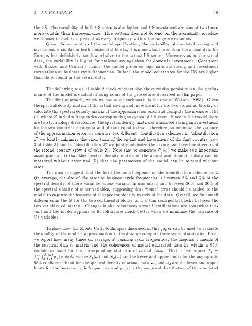
5 AN EXAMPLE 19
the US. The variability of both US series is also higher and US investment are almost two times
more volatile than European ones. This pattern does not depend on the averaging procedure
we choose in fact, it is present atevery frequency within the range we examine.
Given the symmetry of the model speci cation, the variability ofsimulated saving and
investment is similar in both continental blocks, it is somewhat lower than the actual data for
Europe, but de nitively too low relative to the actual US series. Moreover, as in the actual
data, the variability is higher for national savings than for domestic investment. Consistent
with Baxter and Crucini's claims, the model produces high national saving and investment
correlations at business cycle frequencies. In fact, the model coherences for the US are higher
than those found in the actual data.
The following rows of table 2 check whether the above results persist when the performance
of the model is evaluated using some of the procedures described in this paper.
The rst approach, which we use as a benchmark, is the one of Watson (1993). Given
the spectral density matrix of the actual saving and investment for the two economic blocks, we
calculate the spectral density matrix of the approximation error and compute the measure of t
(4) where Z includes frequencies corresponding to cycles of 3-8 years. Since in the model there
are twotechnology disturbances, the spectral density matrix of simulated saving and investment
for the two countries is singular and of rank equal to two. Therefore, to minimize the variance
of the approximation error we consider two di erent identi cation schemes: in \identi cation
1" we jointly minimize the error term of the saving and investment of the rst country (row
3 of table 2) and in \identi cation 2" we jointly minimize the saving and investment errors of
the second country (row 4 of table 2). Note that to generate Rj(!) wemaketwo important
assumptions: (i) that the spectral density matrix of the actual and simulated data can be
measured without error and (ii) that the parameters of the model can be selected without
error.
The results suggest that the t of the model depends on the identi cation scheme used.
On average, the size of the error at business cycle frequencies is between 2% and 5% of the
spectral density of those variables whose variance is minimized and between 20% and 30% of
the spectral density ofothervariables, suggesting that \some" error should be added to the
model to capture the features of the spectral density matrix of the data. Overall, we nd small
di erences in the t for the two continental blocks, and within continental blocks between the
two variables of interest. Changes in the coherences across identi cations are somewhat relevant
and the model appears to t coherences much better when we minimize the variance of
US variables.
To show how the Monte Carlo techniques discussed in this paper can be used to evaluate
the quality of the model's approximation to the data we compute three types of statistics. First,
we report how many times on average, at business cycle frequencies, the diagonal elements of
the spectral density matrix and the coherences of model generated data lie within a 95%
con dence band for the corresponding statistics of actual data. That is, we report T 1 =
R !2
!1
R S2(!)
S1(!) p!(x)dxd! where S 1(!) and S 2(!) are the lower and upper limits for the asymptotic
95% con dence band for the spectral density ofactualdata,! 1 and ! 2 are the lower and upper
limits for the business cycle frequencies and p!(x) is the empirical distribution of the simulated