Testing Calibrated General Equilibrium Models - Universitat ...

5 AN EXAMPLE 21
In sum, this evaluation procedure con rms that the model is better suited in matching
coherences than volatilities at business cycle frequencies and that the covering properties of
the model do not improve when we allow the parameters to be random.
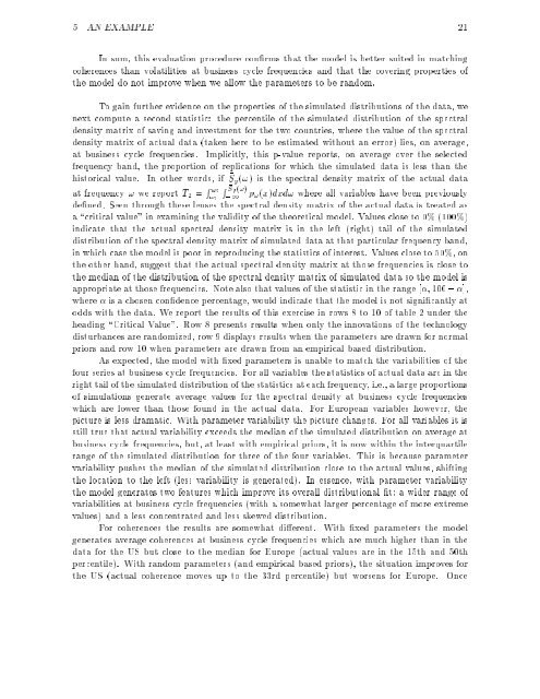
To gain further evidence on the properties of the simulated distributions of the data, we
next compute a second statistic: the percentile of the simulated distribution of the spectral
density matrix of saving and investment for the two countries, where the value of the spectral
density matrix of actual data (taken here to be estimated without an error) lies, on average,
at business cycle frequencies. Implicitly, this p-value reports, on average over the selected
frequency band, the proportion of replications for which the simulated data is less than the
historical value. In other words, if Sy(!) is the spectral density matrix of the actual data
at frequency ! we report T 2 = R !2
!1
R Sy (!)
;1 p!(x)dxd! where all variables have been previously
de ned. Seen through these lenses the spectral density matrix of the actual data is treated as
a \critical value" in examining the validity of the theoretical model. Values close to 0% (100%)
indicate that the actual spectral density matrix is in the left (right) tail of the simulated
distribution of the spectral density matrix of simulated data at that particular frequency band,
in which case the model is poor in reproducing the statistics of interest. Values close to 50%, on
the other hand, suggest that the actual spectral density matrix at those frequencies is close to
the median of the distribution of the spectral density matrixofsimulated data so the model is
appropriate at those frequencies. Note also that values of the statistic in the range [ 100 ; ],
where is a chosen con dence percentage, would indicate that the model is not signi cantly at
odds with the data. We report the results of this exercise in rows 8 to 10 of table 2 under the
heading \Critical Value". Row 8presents results when only the innovations of the technology
disturbances are randomized, row 9 displays results when the parameters are drawn for normal
priors and row 10 when parameters are drawn from an empirical based distribution.
As expected, the model with xed parameters is unable to match the variabilities of the
four series at business cycle frequencies. For all variables the statistics of actual data are in the
right tail of the simulated distribution of the statistics at each frequency, i.e., a large proportions
of simulations generate average values for the spectral density at business cycle frequencies
which arelower than those found in the actual data. For European variables however, the
picture is less dramatic. With parameter variability the picture changes. For all variables it is
still true that actual variability exceeds the median of the simulated distribution on average at
business cycle frequencies, but, at least with empirical priors, it is now within the interquartile
range of the simulated distribution for three of the four variables. This is because parameter
variability pushes the median of the simulated distribution close to the actual values, shifting
the location to the left (less variability is generated). In essence, with parameter variability
the model generates two features which improve itsoverall distributional t: a wider range of
variabilities at business cycle frequencies (with a somewhat larger percentage of more extreme
values) and a less concentrated and less skewed distribution.
For coherences the results are somewhat di erent. With xed parameters the model
generates average coherences at business cycle frequencies which aremuch higher than in the
data for the US but close to the median for Europe (actual values are in the 15th and 50th
percentile). With random parameters (and empirical based priors), the situation improves for
the US (actual coherence moves up to the 33rd percentile) but worsens for Europe. Once