Testing Calibrated General Equilibrium Models - Universitat ...
Testing Calibrated General Equilibrium Models - Universitat ...
Testing Calibrated General Equilibrium Models - Universitat ...

Create successful ePaper yourself
Turn your PDF publications into a flip-book with our unique Google optimized e-Paper software.
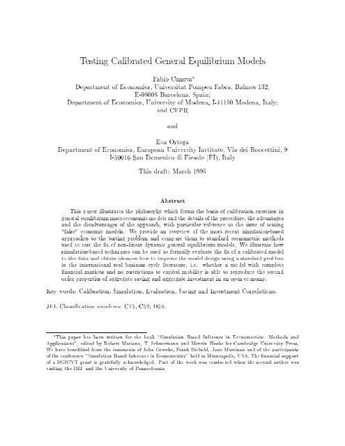
<strong>Testing</strong> <strong>Calibrated</strong> <strong>General</strong> <strong>Equilibrium</strong> <strong>Models</strong><br />
Fabio Canova<br />
Department of Economics, <strong>Universitat</strong> Pompeu Fabra, Balmes 132,<br />
E-08008 Barcelona, Spain<br />
Department of Economics, University of Modena, I-41100 Modena, Italy<br />
and CEPR<br />
and<br />
Eva Ortega<br />
Department of Economics, European University Institute, Via dei Roccettini, 9<br />
I-50016 San Domenico di Fiesole (FI), Italy<br />
This draft: March 1996<br />
Abstract<br />
This paper illustrates the philosophy which forms the basis of calibration exercises in<br />
general equilibrium macroeconomic models and the details of the procedure, the advantages<br />
and the disadvantages of the approach, with particular reference to the issue of testing<br />
\false" economic models. We provide an overview of the most recent simulation-based<br />
approaches to the testing problem and compare them to standard econometric methods<br />
used to test the t of non-linear dynamic general equilibrium models. We illustrate how<br />
simulation-based techniques can be used to formally evaluate the t of a calibrated model<br />
to the data and obtain ideas on how toimprove the model design using a standard problem<br />
in the international real business cycle literature, i.e. whether a model with complete<br />
nancial markets and no restrictions to capital mobility is able to reproduce the second<br />
order properties of aggregate saving and aggregate investment in an open economy.<br />
Key words: Calibration, Simulation, Evaluation, Saving and Investment Correlations.<br />
JEL Classi cation numbers: C15, C52, D58.<br />
This paper has been written for the book \Simulation Based Inference in Econometrics: Methods and<br />
Applications", edited by Robert Mariano, T. Schuermann and Mervin Weeks for Cambridge University Press.<br />
We have bene tted from the comments of John Geweke, Frank Diebold, Jane Marrinan and of the participants<br />
of the conference "Simulation Based Inference in Econometrics" held in Minneapolis, USA. The nancial support<br />
of a DGICYT grant is gratefully acknowledged. Part of the work was conducted when the second author was<br />
visiting the IMF and the University ofPennsylvania
1 INTRODUCTION 1<br />
1 Introduction<br />
Simulation techniques are now used in many elds of applied research. As shown elsewhere<br />
in this book, they have been employed to compute estimators in situations where standard<br />
methods are impractical or fail, to evaluate the properties of parametric and nonparametric<br />
econometric estimators, to provideacheap way ofevaluating posterior integrals in Bayesian<br />
analysis and to undertake linear and nonlinear ltering with a computationally simple approach.<br />
Thetaskofthischapter is to describe how simulation based methods can be used to evaluate<br />
the t of dynamic general equilibrium models speci ed using a calibration methodology,<br />
to compare and contrast their usefulness relative to more standard econometric approaches and<br />
to provide an explicit example where the various features of the approach can be highlighted<br />
and discussed.<br />
The structure of this chapter is as follows. First, we provide a de nition of what we mean<br />
by calibrating a model and discuss the philosophy underlying the approach and how it di ers<br />
from standard dynamic time series modelling. Second, we discuss various approaches to the<br />
selection of model parameters, how tochoose the vector of statistics used to compare actual<br />
with simulated data and how simulations are performed. Third, we describe how to formally<br />
evaluate the model's approximation to the data and discuss alternative approaches to account<br />
for the uncertainty faced by a simulator in generating time paths for the relevant variables.<br />
Although we present a general overview of alternative evaluation techniques, the focus is on<br />
simulation based methods. Finally, we present an example, borrowed from Baxter and Crucini<br />
(1993), where the features of the various approaches to evaluation can be examined.<br />
2 What is Calibration?<br />
2.1 A De nition<br />
Although it is more than a decade since calibration techniques emerged in the main stream<br />
of dynamic macroeconomics (see Kydland and Prescott (1982)), a precise statement of what<br />
it means to calibrate a model has yet to appear in the literature. In general, it is common to<br />
think of calibration as an unorthodox procedure to select the parameters of a model. This need<br />
not to be the case since it is possible to view parameter calibration as a particular econometric<br />
technique where the parameters of the model are estimated using an \economic" instead of a<br />
\statistical" criteria (see e.g. Canova (1994)). On the other hand, one may want to calibrate<br />
a model because there is no available data to estimate its parameters, for example, if one is<br />
interested in studying the e ect of certain taxes in a newly born country.<br />
Alternatively, it is possible to view calibration as a cheap way toevaluate models. For<br />
example, calibration is considered by some a more formal version of the standard back-ofthe-envelope<br />
calculations that theorists perform to judge the validity of their models (see e.g.<br />
Pesaran and Smith (1992)). According to others, calibration is a way to conduct quantitative<br />
experiments using models which are known to be \false", i.e. improper or simpli ed approximations<br />
of the true data generating processes of the actual data (see e.g. Kydland and Prescott<br />
(1991)).<br />
Pagan (1994) stresses that the unique feature of calibration exercises does not lie so
2 WHAT IS CALIBRATION? 2<br />
much in the way parameters are estimated, as the literature has provided alternative ways of<br />
doing so, but in the particular collection of procedures used to test tightly speci ed (and false)<br />
theoretical models against particular empirical facts. Here we takeamoregeneralpointof<br />
view and identify 6 steps which we believe capture the essence of the methodology. We call<br />
calibration a procedure which involves:<br />
(i) Formulating an economic question to be addressed.<br />
(ii) Selecting a model design which bears some relevance to the question asked.<br />
(iii) Choosing functional forms for the primitives of the model and nding a solution for the<br />
endogenous variables in terms of the exogenous variables and the parameters.<br />
(iv) Choosing parameters and stochastic processes for the exogenous variables and simulating<br />
paths for the endogenous variables of the model.<br />
(v) Selecting a metric and comparing the outcomes of the model relative to a set of \stylized<br />
facts".<br />
(vi) Doing policy analyses if required.<br />
By \stylized facts" the literature typically means a collection of sample statistics of the<br />
actual data such as means, variances, correlations, etc., which (a) do not involve estimation<br />
of parameters and (b) are self-evident. More recently, however, the rst requirement has been<br />
waived and the parameters of a VAR (or the impulse responses) have also been taken as the<br />
relevant stylized facts to be matched by the model (see e.g. Smith (1993), Cogley and Nason<br />
(1994)).<br />
The next two subsections describe in details both the philosophy behind the rst four<br />
steps and the practicalities connected with their implementation.<br />
2.2 Formulating a question and choosing a model<br />
The rst two steps of a calibration procedure, to formulate a question of interest and a model<br />
which bears relevance to the question, are self evident and require little discussion. In general,<br />
the questions posed display four types of structure (see e.g. Kollintzas (1992) and Kydland<br />
(1992)):<br />
Is it possible to generate Z using theory W?<br />
How much of the fact X can be explained with impulses of type Y?<br />
What happens to the endogenous variables of the model if the stochastic process for the<br />
control variable V is modi ed ?<br />
Is it possible to reduce the discrepancy D of the theory from the data by introducing<br />
feature F in the model?
2 WHAT IS CALIBRATION? 3<br />
Two economic questions which have received considerable attention in the literature in the last<br />
10 years are the so-called equity premium puzzle, i.e. the inability of a general equilibrium<br />
model with complete nancial markets to quantitatively replicate the excess returns of equities<br />
over bonds over the last hundred years (see e.g. Mehra and Prescott (1985)) and how much<br />
of the variability of GNP can be explained by a model whose only source of dynamics are<br />
technology disturbances (see e.g. Kydland and Prescott (1982)). As is clear from these two<br />
examples, the type of questions posed are very speci c and the emphasis is on the numerical<br />
implications of the exercise. Generic questions with no numerical quanti cation are not usually<br />
studied in this literature.<br />
For the second step, the choice of an economic model, there are essentially no rules<br />
except that it has to have some relevance with the question asked. For example, if one is<br />
interested in the equity premium puzzle, one can choose a model which isvery simply speci ed<br />
on the international and the government side, but very well speci ed on the nancial side so<br />
that it is possible to calculate the returns on various assets. Typically, one chooses dynamic<br />
general equilibrium models. However, several authors have used model designs coming from<br />
di erent paradigms (see e.g. the neo-keynesian model of Gali (1994), the non-walrasian models<br />
of Danthine and Donaldson (1992) or Gali (1995) and the model with union bargaining of<br />
Eberwin and Kollintzas (1995)). There is nothing in the procedure that restricts the class<br />
of model design to be used. The only requirement is that the question that the researcher<br />
formulates is quanti able within the context of the model and that the theory, in the form of<br />
a model design, is fully speci ed.<br />
It is important to stress that a model is chosen on the basis of the question asked and<br />
not on its being realistic or being able to best replicate the data (see Kydland and Prescott<br />
(1991) or Kydland (1992)). In other words, how well it captures reality is not a criteria to<br />
select models. What is important is not whether a model is realistic or not but whether it is<br />
able to provide a quantitative answer to the speci c question the researcher poses.<br />
This brings us to discuss an important philosophical aspect of the methodology. From<br />
the point of view of a calibrator all models are approximations to the DGP of the data and, as<br />
such, false. This aspect of the problem has been appreciated by several authors even before the<br />
appearance of the seminal article of Kydland and Prescott. For example, Hansen and Sargent<br />
(1979) also concede that an economic model is a false DGP for the data. Because of this and<br />
in order to test the validity of the model using standard statistical tools, they complete the<br />
probabilistic structure of the model by adding additional sources of variability, in the form of<br />
measurement errors or unobservable variables, to the fundamental forces of the economy.<br />
For calibrators, the model is not a null hypothesis to be tested but an approximation of a<br />
few dimensions of the data. A calibrator is not interested in verifying whether the model is true<br />
(the answer is already known from the outstart), but in identifying which aspects of the data<br />
a false model can replicate and whether di erent modelsgive di erent answers because they<br />
are false in di erent dimensions. A calibrator is satis ed with his e ort if, through a process of<br />
theoretical respeci cation, a simple and highly stylized model captures an increasing number of<br />
features of the data (confront this activity with the so-called normal science of Kuhn (1970)).<br />
Being more explicit, consider the realization of a vector of stochastic processes yt (our<br />
data) and some well speci ed theoretical model xt = f(zt ) which has something to say about<br />
yt, where zt are exogenous and predetermined variables and is a parameter vector. Because
2 WHAT IS CALIBRATION? 4<br />
the model does not provide a complete description of the phenomenon under investigation we<br />
write<br />
(1)<br />
yt = xt + ut<br />
where ut is an error representing what is missing from f(zt ) to reproduce the stochastic<br />
process generating yt and whose properties are, in general, unknown (it need not necessarily<br />
be mean zero, serially uncorrelated, uncorrelated with the x's and so on). Let By and Bx<br />
be continuous and di erentiable functions of actual and simulated data, respectively. Then<br />
standard econometric procedures judge the coherence of the model to the data by testing<br />
whether or not Bx = By, given that the di erence between Bx and By and their estimated<br />
counterpart b Bx and b By arise entirely from sampling error. While this is a sensible procedure<br />
when the null hypothesis is expected to represent the data, it is less sensible when it is known<br />
that the model does not completely capture all aspects of the data.<br />
The third step of a calibration exercise concerns the solution of the model. To be able<br />
to obtain quantitative answers from a model it is necessary to nd an explicit solution for<br />
the endogenous variables of the model in terms of the exogenous and predetermined variables<br />
and the parameters. For this reason it is typical to parameterize the objective function of the<br />
agents so that manipulation of the rst order conditions is analytically tractable. For example,<br />
in general equilibrium models, it is typical to choose Cobb-Douglas production functions and<br />
constant relative risk aversion utility functions. However, although the main objective isto<br />
select simple enough functional forms, it is well known that almost all general equilibrium<br />
models and many partial equilibrium models have exact analytical solutions only in very special<br />
situations.<br />
For general equilibrium models, a solution exists if the objective function is quadratic<br />
and the constraints linear (see e.g. Hansen and Sargent (1979)) or when the objective function<br />
is log-linear and the constraints linear (see e.g. Sargent (1987, ch.2)). In the other cases,<br />
analytical expressions relating the endogenous variables of the model to the \states" of the<br />
problem does not exist and it is necessary to resort to numerical techniques to nd solutions<br />
which approximate equilibrium functionals either locally or globally. There has been substantial<br />
theoretical development in this area in the last few years and several solution algorithms have<br />
appeared in the literature (see e.g. the special January 1990 issue of the JBES or Marcet<br />
(1994)).<br />
The essence of the approximation process is very simple. The exact solution of a model is<br />
a relationship between the endogenous variables xt, the exogenous and predetermined variables<br />
zt and a set of \deep" parameters of the type xt = f(zt ) where f is generally unknown.<br />
The approximation procedures generate a relationship of the type x t = g(zt ) where = h( )<br />
and where jjf ; gjj < is minimal for some local or global metric. Examples of these types<br />
of procedures appear in Kydland and Prescott (1982), Coleman (1989), Tauchen and Hussey<br />
(1991), Novales (1990), Baxter (1992) and Marcet (1992), among others. The choice of a<br />
particular approximation procedure depends on the question asked. If one is concerned with<br />
the dynamics of the model around the steady state, local approximations are su cient. On the<br />
other hand, if one is interested in comparing economic policies requiring drastic changes in the<br />
parameters of the control variables, global approximation methods must be preferred.
2 WHAT IS CALIBRATION? 5<br />
2.3 Selecting Parameters and Exogenous Processes<br />
Once an approximate solution has been obtained, a calibrator needs to select the parameters<br />
and the exogenous stochastic process zt to be fed into the model in order to generate time<br />
series for x t . There are several approaches to the choice of these two features of the model.<br />
Consider rst the question of selecting zt. This choice is relatively uncontroversial. One either<br />
chooses it on the basis of tractability or to give the model some realistic connotation. For<br />
example, one can assume that zt is an AR process with innovations which are transformations<br />
of a N(0 1) process and draw one or more realizations for zt using standard random number<br />
generators. Alternatively, one can select the Solow residuals of the actual economy, the actual<br />
path of government expenditure or of the money supply. Obviously, the second alternative is<br />
typically preferred if policy analyses are undertaken. Note that while in both cases zt is the<br />
realization of a stochastic process, in the rst case the DGP is known while in the second it is<br />
not and this has implications for the way one measures the uncertainty in the outcomes of the<br />
model.<br />
Next, consider the selection of the vector of parameters . Typically, they are chosen<br />
so that the model reproduces certain observations. Taking an example from physics, if one is<br />
interested in measuring water temperature in various situations it will be necessary to calibrate<br />
a thermometer for the experiments. For this purpose a researcher arbitrarily assigns the value<br />
0 C to freezing water and the value 100 C to boiling water and interpolates values in the<br />
middle with, say, a linear scale. Given this calibration of the thermometer, one can then<br />
proceed to measure the results of the experiments: avalue close to 100 C indicates \hot"<br />
water, a value close to 30 C indicates \tepid" water, and so on. To try to give answers to<br />
the economic question he poses, a calibrator must similarly select observations to be used to<br />
calibrate the model-thermometer. There are at least three approaches in the literature. One<br />
can follow the deterministic computable general equilibrium (CGE) tradition, summarized,<br />
e.g. in Showen and Walley (1984), the dynamic general equilibrium tradition pioneered by<br />
Kydland and Prescott (1982) or employ more standard econometric techniques. There are<br />
di erences between the rst two approaches. The rstonewas developed for deterministic<br />
models which do not necessarily possess a steady state while the second one has been applied<br />
to dynamic stochastic models whose steady state is unique. Kim and Pagan (1994) provide a<br />
detailed analysis of the di erences between these two approaches. Gregory and Smith (1993)<br />
supplement the discussion by adding interesting insights in the comparison of the rst two<br />
approaches with the third.<br />
In CGE models a researcher solves the model linearizing the system of equations by determining<br />
the endogenous variables around a hypothetical equilibrium where prices and quantities<br />
are such that there is no excess demand or excess supply. It is not necessary that this equilibrium<br />
exists. However, because the coe cients of the linear equations determining endogenous<br />
variables are functions of these equilibrium values, it is necessary to measure this hypothetical<br />
equilibrium. The main problem for this literature is therefore to nd a set of \benchmark<br />
data" and to calibrate the model so that it can reproduce this data. Finding this data set is<br />
the most complicated part of the approach since it requires a lot of judgement and ingenuity.<br />
The process of speci cation of this data set leaves some of the parameters of the model typically<br />
undetermined, for example, those that describe the utility function of agents. In this
2 WHAT IS CALIBRATION? 6<br />
situation a researcher either assigns arbitrary values or xes them to values estimated in other<br />
studies in the literature. Although these choices are arbitrary, the procedure is coherent with<br />
the philosophy of the models: a researcher is interested in examining deviations of the model<br />
from a hypothetical equilibrium, not from an actual economy.<br />
In stochastic general equilibrium models, the model is typically calibrated at the steady<br />
state: parameters are chosen so that the model, in the steady state, produces values for the<br />
endogenous variables which match corresponding long run averages of the actual data. In both<br />
this approach and the CGE approach point estimates of the parameters used to calibrate the<br />
model to the equilibrium are taken to be exact (no standard deviations are typically attached to<br />
these estimates). As in the previous setup, the steady state does not necessarily pin down all the<br />
parameters of the model. Canova (1994) and Gregory and Smith (1993) discuss various methods<br />
to select the remaining parameters. Brie y, a researcher can choose parameters a-priori, pin<br />
them down using values previously estimated in the literature, can informally estimate them<br />
using simple method of moment conditions or formally estimate them using procedures like<br />
GMM (see e.g. Christiano and Eichenbaum (1992)), SMM (see e.g. Du e and Singleton (1993))<br />
or maximum likelihood (see e.g. McGratten, Rogerson and Wright (1993)). As pointed out by<br />
Kydland and Prescott (1991), choosing parameters using the information contained in other<br />
studies imposes a coherence criteria among various branches of the profession. For example,<br />
in the business cycle literature one uses stochastic growth models to examine business cycle<br />
uctuations and checks the implications of the model using parameters typically obtained in<br />
micro studies, which do not employ datahaving to do with aggregate business cycle uctuations<br />
(e.g. micro studies of labor markets).<br />
If one follows a standard econometric approach, all the parameters are chosen by minimizing<br />
the MSE of the error ut in (1), arbitrarily assuming that the error and the model designs<br />
are orthogonal, or by minimizing the distance between moments of the actual data and the<br />
model or maximizing the likelihood function of the data given the model design. As we already<br />
pointed out, this last approach is the least appealing one from the point of view of a calibrator<br />
since it makes assumptions on the time series properties of ut which are hard to justify from<br />
an economic point ofview.<br />
To clearly understand the merits of each of these procedures it is useful to discuss their<br />
advantages and their disadvantages. Both the CGE and the Kydland and Prescott approach<br />
where some of the parameters are chosen a-priori or obtained from a very select group of<br />
studies are problematic in several respects. First, there is a selectivity bias problem (see<br />
Canova (1995)). There exists a great variety of estimates of the parameters in the literature<br />
and di erent researchers may refer to di erent studies even when they are examining the same<br />
problem. Second, there is a statistical inconsistency problem which may generate very spurious<br />
and distorted inference. As Gregory and Smith (1989) haveshown, if some parameters are set apriori<br />
and others estimated by simulation, estimates of the latter may be biased and inconsistent<br />
unless the parameters of the former group are the true parameters of the DGP or consistent<br />
estimates of them. Third, since any particular choice is arbitrary, extensive sensitivity analysis<br />
is necessary to evaluate the quality of the results. To solve these problems Canova (1994)-<br />
(1995) suggests an approach forchoosing parameters which allows, at a second stage, to draw<br />
inferences about the quality of the approximation of the model to the data. The idea is<br />
very simple. Instead of choosing one set of parameters over another he suggests calibrating
2 WHAT IS CALIBRATION? 7<br />
each parameter of the model to an interval, using the empirical information to construct a<br />
distribution over this interval (the likelihood of a parameter given existing estimates) and<br />
conducting simulation by drawing parameter vectors from the corresponding joint \empirical"<br />
distribution. An example may clarify the approach. If one of the parameters of interest is the<br />
coe cient of constant relative risk aversion of the representative agent, one typically chooses<br />
avalue of 2 and tries a few values above andbelow this one to see if results change. Canova<br />
suggests taking a range of values, possibly dictated by economic theory, say [0,20], and then<br />
over this range constructing a histogram using existing estimates of this parameter. Most of the<br />
estimates are in the range [1,2] and in some asset pricing models researchers have tried values<br />
up to 10. Given this information, the resulting empirical distribution for this parameter can<br />
be very closely approximated by a 2 (2), which has the mode at 2 and about 5% probability<br />
in the region above 6.<br />
The selection of the parameters of theoretical models through statistical estimation has<br />
advantages and disadvantages. The main advantage is that these procedures avoid arbitrary<br />
choices and explicitly provide a measure of dispersion for the estimates which can be used at<br />
a second stage to evaluate the quality of the approximation of the model to the data. The<br />
disadvantages are of various kinds. First of all, to undertake a formal or informal estimation<br />
it is typically necessary to select the moments one wants to t, and this choice is arbitrary.<br />
The standard approach suggested by Kydland and Prescott can indeed be thought ofasa<br />
method of moment estimation where one chooses parameters so as to set only the discrepancy<br />
between the rst moment of the model and the data (i.e. the long run averages) to zero. The<br />
formal approach suggested by Christiano and Eichenbaum (1992) or Langot and Feve (1994),<br />
on the other hand, can be thought ofasamethodofmoment estimation where a researcher<br />
ts the discrepancies between model and data rst and second moments to zero. The approach<br />
of choosing parameters by setting to zero the discrepancy between certain moments has the<br />
disadvantage of reducing the number of moments over which it will be possible to evaluate<br />
the quality of the model. Moreover, it is known that estimates obtained with the method of<br />
moments or GMM may be biased. Therefore, simulations and inference conducted with these<br />
estimates may lead to spurious inference (see e.g. Canova, Finn and Pagan (1994)). In addition,<br />
informal SMM may lead one to select parameters even though they are not identi able (see<br />
Gregory and Smith (1989)). Finally, one should note that the type of uncertainty which is<br />
imposed on the model via an estimation process does not necessarily re ect the uncertainty<br />
a calibrator faces when choosing the parameter vector. As is clear from a decade of GMM<br />
estimation, once the moments are selected and the data given, sample uncertainty is pretty<br />
small. The true uncertainty is in the choice of moments and in the data set to be used to select<br />
parameters. This uncertainty is disregarded when parameters are chosen using extremum<br />
estimators like GMM.<br />
Finally, it is useful to compare the parameter selection process used by a calibrator a-la<br />
Kydland and Prescott and the one used by a traditional econometric approach. In a traditional<br />
econometric approach parameters are chosen so as to minimize some statistical criteria, for<br />
example, the MSE. Such criteria do not have any economic content, impose stringent requirements<br />
on the structure of ut and are used, primarily, because there exists a well established<br />
statistical and mathematical literature on the subject. In other words, the parameter selection<br />
criteria used by traditional econometricians does not have economic justi cation. On the
3 EVALUATING CALIBRATED MODELS 8<br />
other hand, the parameter selection criteria used by followers of the Kydland and Prescott<br />
methodology can be thought of as being based on economic criteria. For example, if the<br />
model is calibrated so that, in the steady state, it matches the long run features of the actual<br />
economy, parameters are implicitly selected using the condition that the sum (over time) of<br />
the discrepancies between the model and the data is zero. In this sense there is an important<br />
di erence between the two approaches which has to do with the assumptions that one is willing<br />
to make ontheerrorsut. By calibrating the model to long run observations a researcher selects<br />
parameters assuming E(u) = 0 , i.e. using a restriction which is identical to the one imposed<br />
by a GMM econometrician who chooses parameters using only rst moment conditions. On<br />
the other hand, to conduct classical inference a researcher imposes restrictions on the rst and<br />
second moments of ut.<br />
The comparison we have made so far concerns, obviously, only those parameters which<br />
enter the steady state conditions of the model. For the other parameters a direct comparison<br />
with standard econometric practice is not possible. However, if all parameters are calibrated<br />
to intervals with distributions which are empirically determined, the calibration procedure we<br />
have described shares a tight connection with Bayesian inferential methods such as Consensus<br />
Analysis or Meta-Analysis (see e.g. Genest and Zidak (1986) or Wolf (1986)).<br />
Once the parameters and the stochastic processes for the exogenous variables are selected<br />
and an (approximate) solution to the model has been found, simulated paths for x t can be<br />
generated using standard Monte Carlo simulation techniques.<br />
3 Evaluating <strong>Calibrated</strong> <strong>Models</strong><br />
The questions of how well a model matches the data and how much con dence a researcher<br />
ought togive to the results constitute the most crucial steps in the calibration procedure. In<br />
fact, the most active methodological branch of this literature concerns methods to evaluate the<br />
t of a model selected according to the procedures described in section 2. The evaluation of a<br />
model requires three steps: rst, the selection of a set of stylized facts second, the choice of a<br />
metric to compare functions of actual and simulated data and third, the (statistical) evaluation<br />
of the magnitude of the distance. Formally, letSy be a set of statistics (stylized facts) of the<br />
actual data and let Sx (zt ) be a set of statistics of simulated data, given a vector of parameters<br />
and a vector of stochastic processes zt. Then model evaluation consists of selecting a function<br />
(SySx (zt )) measuring the distance between Sy and Sx and in assessing its magnitude.<br />
The choice of which stylized facts one wants to match obviously depends on the question<br />
asked and on the type of model used. For example, if the question is what is the proportion<br />
of actual cyclical uctuations in GNP and consumption explained by the model, one would<br />
choose stylized facts based on variances and covariances of the data. As an alternative tothe<br />
examination of second moments, one could summarize the properties of actual data via a VAR<br />
and study the properties of simulated data, for example, by comparing the number of unit roots<br />
in the two sets of data (as in Canova, Finn and Pagan (1994)), the size of VAR coe cients<br />
(as in Smith (1993)) or the magnitude of certain impulse responses (as in Cogley and Nason<br />
(1994)). Also, it is possible to evaluate the discrepancy of a model to the data by choosing<br />
speci c events that one wants the model to replicate e.g., business cycle turning points, (as in<br />
King and Plosser (1994) or Simkins (1994)) or variance bounds (as in Hansen and Jagannathan
3 EVALUATING CALIBRATED MODELS 9<br />
(1991)).<br />
Classical pieces in the calibration literature (see e.g. Kydland and Prescott (1982) or<br />
(1991)) are typically silent on the metric one should use to evaluate the quality of the approximation<br />
of the model to the data. The approach favored by most calibrators is to glare over the<br />
exact de nition of the metric used and informally assess the properties of simulated data by<br />
comparing them to the set of stylized facts. In this way a researcher treats the computational<br />
experiment as a measurement exercise where the task is to gauge the proportion of some observed<br />
statistics reproduced by the theoretical model. This informal approach is also shared by<br />
cliometricians (see e.g. Summers (1991)) who believe that rough reproduction of simple sample<br />
statistics is all that is needed to evaluate the implications of the model (\either you see it with<br />
naked eyes or no fancy econometric procedure will nd it").<br />
There are, however, alternatives to this informal approach. To gain some understanding<br />
of the di erences among approaches, but at the cost of oversimplifying the matter, we divide<br />
evaluation approaches into ve classes:<br />
Informal approaches.<br />
Approaches which do not consider sampling variability of actual or the uncertainty in<br />
simulated data, but instead use the statistical properties of ut in (1) to impose restrictions<br />
on the time series properties of . This allows them to provide an R 2 -type measure of t<br />
between the model and the data (see Watson (1993)).<br />
Approaches which use the sampling variability oftheactual data (a ecting Sy and, in<br />
some cases, estimated )toprovide a measure of the distance between the model and<br />
the data. Among these we list the GMM based approach of Christiano and Eichenbaum<br />
(1992), Cecchetti, Lam and Mark (1993) or Feve and Langot (1994), and the frequency<br />
domain approaches of Diebold, Ohanian and Berkowitz (1995) and Ortega (1995).<br />
Approaches which use the uncertainty ofthesimulated data to provide a measure of<br />
distance between the model and the data. Among these procedures we can distinguish<br />
those who take zt as stochastic and as given, such as Gregory and Smith (1991),<br />
Soderlind (1994) or Cogley and Nason (1994) and those who take both zt and as<br />
stochastic, such as Canova (1994) and (1995).<br />
Finally, approaches which consider the sampling variability of the actual data and the<br />
uncertainty insimulated data to evaluate the t of the model. Once again we can<br />
distinguish approaches which, in addition to taking Sy as random, allow for variability in<br />
the parameters of the model (keeping zt xed) such as DeJong, Ingram and Whiteman<br />
(1995) from those which allow for both zt and to vary such asCanova and De Nicolo<br />
(1995).<br />
Because the emphasis of this book is on simulation techniques, we will only brie y examine<br />
the rst three approaches and discuss in more detail the last two, which make extensive use<br />
of simulation techniques to conduct inference. Kim and Pagan (1994) provide a thorough critical<br />
review of several of these evaluation techniques and additional insights on the relationship<br />
among them.
3 EVALUATING CALIBRATED MODELS 10<br />
The evaluation criteria that each of these approaches proposes is tightly linked to the<br />
parameter selection procedure we discussed in the previous section.<br />
As mentioned the standard approach istochoose parameters using steady state conditions.<br />
Those parameters which do not appear in the steady state are selected a-priori or with<br />
reference to existing literature. Also, since Sy is chosen to be a vector of numbers and no<br />
uncertainty isallowed in the selected parameter vector, one is forced to use an informal metric<br />
to compare the model to the data. This is because, apart from the uncertainty present inthe<br />
exogenous variables, the model links the endogenous variables to the parameters in a deterministic<br />
fashion. Therefore, once we have selected the parameters and we have a realization<br />
of Sy, it is not possible to measure the dispersion of the distance (SySx (zt )). >From the<br />
point of view of the majority of calibrators this is not a problem. As emphasized by Kydland<br />
and Prescott (1991) or Kydland (1992), the trust a researcher has in an answer given by the<br />
model does not depend on a statistical measure of discrepancy, but on how much he believes<br />
in the economic theory used and in the measurement undertaken.<br />
Taking this as the starting point of the analysis Watson (1993) suggests an ingenious<br />
way toevaluate models which are known to be an incorrect DGP for the actual data. Watson<br />
asks how much error should be added to x t so that its autocovariance function equals the<br />
autocovariance function of yt. Writing yt = x t + u t where u t includes the approximation error<br />
due to the use x t in place of xt, the autocovariance function of this error is given by<br />
Au (z) =Ay(z)+Ax (z) ; Ax y(z) ; Ayx (z) (2)<br />
To evaluate the last two terms in (2) we need a sample from the joint distribution of (x t yt)<br />
which is not available. In these circumstances it is typical to assume that either u t is a<br />
measurement error or a signal extraction noise (see e.g. Sargent (1989)), but in the present<br />
context neither of the two assumptions is very appealing. Watson suggests choosing Ax y(z) so<br />
as to minimize the variance of u t subject to the constraint that Ax (z) andAy(z) are positive<br />
semide nite. Intuitively, the idea is to select Ax y(z) togive the best possible t between the<br />
model and the data (i.e. the smallest possible variance of u t ). The exact choice of Ax y(z)<br />
depends on the properties of x t and yt, i.e. whether they are serially correlated or not, scalar or<br />
vectors, full rank processes or not. In all cases, the selection criteria chosen imply that x t and<br />
yt are perfectly linearly correlated where the matrix linking the two vectors depends on their<br />
time series properties and on the number of shocks bu eting the model. Given this framework<br />
of analysis, Watson suggests two measures of t, similar to a 1 ; R 2 from a regression, of the<br />
form<br />
rj(!) = Au (!)jj<br />
Ay(!)jj<br />
Rj(!) =<br />
R<br />
!2Z<br />
Au (!)jjd!<br />
R<br />
!2Z Ay(!)jjd!<br />
where the rst statistic measures the variance of the j-th component of the error relative to<br />
the variance of the j-th component of the data for each frequency and the second statistic is<br />
the sum of the rst over a set of frequencies. This last measure may be useful to evaluate<br />
the model, say, at business cycle frequencies. It should be stressed that (3) and (4) are lower<br />
(3)<br />
(4)
3 EVALUATING CALIBRATED MODELS 11<br />
bounds. That is, when rj(!) orRj(!) are large, the model poorly ts the data. However, when<br />
they are small, it does not necessarily follow that the model is appropriate since it may still t<br />
the data poorly if we change the assumptions about Ax y(z).<br />
To summarize, Watson chooses the autocovariance function of y as the set of stylized<br />
facts of the data to be matched by the model, the function as the ratio of Au to Ay and<br />
evaluates the size of informally (i.e. if it is greater than one, between zero and one or close<br />
to zero). Note that in this approach, and zt are xed, and Ax and Ay are assumed to be<br />
measured without error.<br />
When a calibrator is willing to assume that parameters are measured with error because,<br />
given an econometric technique and a sample, parameters are imprecisely estimated, then model<br />
evaluation can be conducted using measures of dispersion for simulated statistics which re ect<br />
parameter uncertainty. There are various versions of this approach. Christiano and Eichenbaum<br />
(1992), Cecchetti, Lam and Mark (1993) and Feve and Langot (1994) use a version of a J-test<br />
to evaluate the t of a model. In this case Sy are moments of the data while is a quadratic<br />
function of the type<br />
(SySx (zt )) = [Sy ; Sx ( )]V ;1 [Sy ; Sx ( )] 0<br />
where V is a matrix which linearly weights the covariance matrix of Sx and Sy, andSx is<br />
random because is random. Formal evaluation of this distance can be undertaken following<br />
Hansen (1982): under the null that Sy = Sx (zt ) the statistic de ned in (5) is asymptotically<br />
distributed as a 2 with the number of degrees of freedom equal to the numberofoveridentifying<br />
restrictions, i.e. the dimension of Sy minus the dimension of the vector . Note that this<br />
procedure is correct asymptotically, that it implicitly assumes that xt = f(zt ) (or its approximation<br />
xt ) is the correct DGP for the data and that the relevant loss function measuring the<br />
distance between actual and simulated data is quadratic.<br />
The methods proposed by Diebold, Ohanian and Berkowitz (DOB) (1994) and Ortega<br />
(1995) are slightly di erent but can be broadly included into this class of approaches.<br />
For DOB the statistic of interest is the spectral density matrix of yt and, given a sample,<br />
this is assumed to be measured with error. They measure the uncertainty surrounding point<br />
estimates of the spectral density matrix employing (small sample) 90% con dence bands constructed<br />
using parametric and nonparametric bootstrap approaches and Bonferroni tunnels.<br />
On the other hand, they take calibrated parameters and the realization of zt as given so that<br />
the spectral density matrix of simulated data can be estimated without error simply by simulating<br />
very long time series for xt . Ortega (1995) also takes the spectral density matrix as the<br />
set of stylized facts of the data to be matched by the model. Unlike DOB, she considers the<br />
uncertainty in actual and simulated data by jointly estimating the spectral density matrix of<br />
actual and simulated data and constructs measures of uncertainty around point estimates of<br />
the spectral density matrix using asymptotic distribution theory.<br />
In both cases, the measure of t used is generically given by:<br />
C( zt) =<br />
Z<br />
0<br />
(5)<br />
(Fy(!)Fx (! zt))W (!)d! (6)<br />
where W (!) is a set of weights applied to di erent frequencies and F are the spectral density<br />
matrices of actual and simulated data.
3 EVALUATING CALIBRATED MODELS 12<br />
DOB suggest various options for (quadratic, ratio, likelihood type) but do not construct<br />
a direct test statistic to examine the magnitude of . Instead, they compute a small sample<br />
distribution of the event that C( zt) is close to a particular value (zero if is quadratic, 1 if<br />
is a ratio, etc.) Ortega, on the other hand, explicitly uses a quadratic expression for and uses<br />
an asymptotic 2 test to assess whether the magnitude of the discrepancy between the model<br />
and the data is signi cant or not. The set of asymptotic tools she develops can also be used<br />
to compare the t of two alternative models to the data and decide which one is more acceptable.<br />
If a calibrator is willing to accept the idea that the stochastic process for the exogenous<br />
variables is not xed, she can then compute measures of dispersion for simulated statistics by<br />
simply changing the realization of zt while maintaining the parameters xed. Such a methodology<br />
has its cornerstone in the fact that it is the uncertainty in the realization of the exogenous<br />
stochastic process (e.g. the technology shock), an uncertainty which one can call extrinsic, and<br />
not the uncertainty in the parameters, which one can call intrinsic, which determines possible<br />
variations in the statistics of simulated data. Once a measure of dispersion of simulated statistics<br />
is obtained, the sampling variability of simulated data can be used to evaluate the distance<br />
between statistics of actual and simulated data (as e.g. Gregory and Smith (1991) and (1993)).<br />
If one uses such anapproach, model evaluation can be undertaken with a probabilistic<br />
metric using well known Monte Carlo techniques. For example, one maybeinterested in nding<br />
out in what decile of the simulated distribution the actual value of a particular statistic lies,<br />
in practice, calculating the \size" of calibration tests. This approach requires two important<br />
assumptions: that the evaluator takes the model economy as the true DGP for the data and<br />
that di erences between Sy and Sx occur only because of sampling variability. To be speci c,<br />
Gregory and Smith take Sy be a set of moments of the data and assume that they can be measured<br />
without error. Then, they construct a distribution of Sx (zt )bydrawing realizations<br />
for the zt process from a given distribution, given . The metric used is probabilistic, i.e.<br />
they calculate the probability Q = P (Sx Sy), and judge the t of the model informally, e.g.<br />
measuring how closeQ is to 0.5.<br />
An interesting variation on this setup is provided by Soderlind (1994) and Cogley and<br />
Nason (1994). Soderlind employs the spectral density matrix of the actual data while Cogley<br />
and Nason choose a \structural" impulse response function as the relevant statistics to be<br />
matched. Soderlind maintains a probabilistic metric and constructs the empirical rejection<br />
rate for the event that the actual spectral density matrixof yt lies inside the asymptotic<br />
90% con dence band for the spectral density matrix of the simulated data. Such anevent is<br />
replicated by drawing vectors zt for a given distribution. Cogley and Nason choose a quadratic<br />
measure of distance which, under the null that the model is the DGP for the data, has an<br />
asymptotic 2 distribution and then tabulate the empirical rejection rates of the test, by<br />
repeatedly constructing the statistic drawing realizations of the zt vector. To be speci c, the<br />
function is in this case given by<br />
kj( )=[IRF k x (z j<br />
t ) ; IRFk y ]V ;1 [IRF k x (z j<br />
t ) ; IRFk y ] 0<br />
where j indexes replications and k steps, IRF k is the impulse response function and V is<br />
its asymptotic covariance matrix at step k. Because for every k and for xed j kj( )is<br />
(7)
3 EVALUATING CALIBRATED MODELS 13<br />
asymptotically 2 , they can construct (a) the simulated distribution for kj and compare it<br />
with a 2 and (b) the rejection frequency for each model speci cation they examine.<br />
In practice, all three approaches are computer intensive and rely on Monte Carlo methods<br />
to conduct inference. Also, it should be stressed that all three methods verify the validity<br />
of the model by computing the \size" of the calibration tests, i.e. assuming that the model is<br />
the correct DGP for yt.<br />
The approach of Canova (1994)-(1995) also belongs to this category of methods, but,<br />
in addition to allowing the realization of the stochastic process for the exogenous variables to<br />
vary, he also allows for parameter variability in measuring the dispersion of simulated statistics.<br />
The starting point, as discussed earlier, is that parameters are uncertain not so much because<br />
of sample variability, but because there are many estimates of the same parameter obtained in<br />
the literature, since estimation techniques, samples and frequency of the data tend to di er. If<br />
one calibrates the parameter vector to an interval, rather than to a particular value, and draws<br />
values for the parameters from the empirical distribution of parameter estimates, it is then possible<br />
to use the intrinsic uncertainty, in addition to or instead of the extrinsic one, to evaluate<br />
the t of the model. The evaluation approach usedisvery similar to the one of Gregory and<br />
Smith: one simulates the model repeatedly by drawing parameter vectors from the empirical<br />
\prior" distribution and realizations of the exogenous stochastic process zt from some given<br />
distribution. Once the empirical distribution of the statistics of interest is constructed, one can<br />
then compute either the size of calibration tests or the percentiles where the actual statistics lie.<br />
The last set of approaches considers the uncertainty present in the statistics of both<br />
actual and simulated data to measure the t of the model to the data. In essence what<br />
these approaches attempt to formally measure is the degree of overlap between the (possibly)<br />
multivariate distributions of Sy and Sx using Monte Carlo techniques. There are di erences<br />
in the way these distributions have been constructed in the literature. Canova and De Nicolo<br />
(1995) use a parametric bootstrap algorithm to construct distributions for the statistics of<br />
the actual data . DeJong, Ingram and Whiteman (DIW) (1995), on the other hand, suggest<br />
representing the actual data with a VAR and computing posterior distribution estimates for the<br />
moments of interest by drawing VAR parameters from their posterior distribution and using<br />
the AR(1) companion matrix of the VAR at each replication. In constructing distributions of<br />
simulated statistics, Canova and De Nicolo takeinto account both the uncertainty in exogenous<br />
processes and parameters while DIW only consider parameter uncertainty. The two approaches<br />
also di er in the way the \prior" uncertainty in the parameters is introduced in the model. The<br />
former paper follows Canova (1995) and chooses empirical based distributions for the parameter<br />
vector. DIW use subjectively speci ed prior distributions (generally normal) whose location<br />
parameter is set at the value typically calibrated in the literature while the dispersion parameter<br />
is free. The authors use this parameter in order to (informally) minimize the distance between<br />
actual and simulated distributions of the statistics of interest. By enabling the speci cation of<br />
a sequence of increasingly di use priors over the parameter vector, such a procedure illustrates<br />
whether the uncertainty in the model's parameters can mitigate di erences between the model<br />
and the data.<br />
Finally, there are di erences in assessing the degree of overlap of the two distributions.
3 EVALUATING CALIBRATED MODELS 14<br />
Canova and De Nicolo choose a particular contour probability for one of the two distributions<br />
and ask how much of the other distribution is inside the contour. In other words, the t of<br />
the model is examined very much in the style of the Monte Carlo literature: a good t is<br />
indicated by a high probability covering of the two regions. To describe the features of the<br />
two distributions, they also repeat the exercise varying the chosen contour probability, say,<br />
from 50% to 75%, 90%, 95% and 99%. The procedure allows them to detect anomalies in<br />
the shape of the two distributions due to clustering of observations in one area, skewness or<br />
leptokurtic behavior. In this approach actual data and simulated data are used symmetrically<br />
in the sense that one can either ask whether the actual data could be generated by the model, or<br />
viceversa, whether simulated data are consistent with the distribution of the empirical sample.<br />
This symmetry allows the researcher to understand much better the distributional properties of<br />
error ut in (1). Moreover, the symmetry with which the two distributions are treated resembles<br />
very much the process of switching the null and the alternative in standard classical hypothesis<br />
testing.<br />
DeJong, Ingram and Whiteman take the point of view that there are no well established<br />
criteria to judge the adequacy of a model's \approximation" to reality. For this reason they<br />
present two statistics aimed at synthetically measuring the degree of overlap among distributions.<br />
One, which they call Con dence Interval Criterion (CIC) is the univariate version of the<br />
contour probability criteria used by Canova and De Nicolo and is de ned as<br />
CICij = 1<br />
1 ;<br />
Z b<br />
a<br />
Pj(si)dsi<br />
where si i =1:::n is a set of functions of interest, a = and b =1; a are the quantiles<br />
2<br />
of D(si), the distribution of the statistic in the actual data, Pj(si) is the distribution of the<br />
simulated statistic where j is the di usion index of the prior on the parameter vector and<br />
1 ; = R b<br />
a D(si)dsi. Note that with this de nition, CICij ranges between 0 and 1<br />
1; . For<br />
CIC close to zero, the t of the model is poor, either because the overlap is small or because<br />
Pj is very di use. For CIC close to 1<br />
1; the two distributions overlap substantially. Finally, if<br />
CIC > 1, D(si) is di use relative toPj(si), i.e. the data is found to be relatively uninformative<br />
regarding si.<br />
To distinguish among the two possible interpretations when CIC is close to zero, DeJong,<br />
Ingram and Whiteman suggest a second summary measure analogous to a t-statistic for the<br />
mean of Pj(si) in the D(si) distribution, i.e.,<br />
dji = EPj(si) ; ED(si)<br />
p<br />
varD(si)<br />
Large values of (9) indicate that the location of Pj(si) isquitedi erent from the location of<br />
D(si).<br />
The nal problem of the DIW methodology is to choose . DeJong, Ingram and Whiteman<br />
x a particular value ( =0:01) but, as in Canova and De Nicolo, varying for a given<br />
j is probably a good thing to do in order to describe the feature of the distributions. This is<br />
particularly useful when we areinterested in partitions of the joint distributions of si because<br />
graphical methods or simple statistics are not particularly informative about distributions in<br />
high dimensional spaces.<br />
(8)<br />
(9)
4 POLICY ANALYSES 15<br />
4 Policy Analyses<br />
Although it is not the purpose of this chapter to discuss in detail how calibrated models can be<br />
used for policy analyses, it is useful to describe the implications of the procedure for questions<br />
which have policy implications and how policy experiments can be undertaken. As we have<br />
already mentioned, a model is typically calibrated to provide a quantitative answer to very<br />
precise questions and some of these questions have potential policy implications. To forcefully<br />
argue the policy implications of the exercise one needs to be con dent in the answer given by<br />
the model and to do this it is necessary to undertake extensive sensitivity analysis to check<br />
how results change when certain assumptions are modi ed.<br />
As we have seen, the answers of the model come in the form of continuous functions<br />
h(x t )=h(g(zt )) of simulated data. In theory, once g has been selected, the uncertainty inh<br />
is due to the uncertainty in and in zt. Since in standard calibration exercises the vector is<br />
xed, it is therefore typical to examine the sensitivity of the results in the neighborhood of the<br />
calibrated values for . Such experiments may be local, if the neighborhood is small, or global,<br />
in which case one measures the sensitivity of the results to perturbations of the parameters<br />
over the entire range. This type of exercise may provide two types of information. First, if<br />
results are robust to variations of a parameter in a particular range, its exact measurement is<br />
not crucial. In other words, the uncertainty present in the choice of such a parameter does not<br />
make the answers of the model tenuous and economic inference groundless. On the other hand,<br />
if results crucially depend on the exact selection of certain parameters, it is clearly necessary<br />
to improve upon existing measurement of these parameters.<br />
A local sensitivity analysis can be undertaken informally, replicating the experiments<br />
for di erent values of the parameters (as in Kydland and Prescott (1982)) or more formally,<br />
calculating the elasticity ofh with respect to (as in Pagan and Shannon (1985)). A global<br />
sensitivity analysis can be e ciently undertaken with Monte Carlo methods or numerical semideterministic<br />
techniques (see e.g. Niederreiter (1988)) if the function g is known and the<br />
distribution of the vector is speci ed. If g is only an approximation to the functional linking<br />
x to z and , one can use techniques like Importance Sampling (see Geweke (1989)) to takeinto<br />
account this additional source of uncertainty. Clearly the two types of sensitivity analysis are<br />
not incompatible and should both be undertaken to assess the degree of trust a researcher can<br />
attach to the answer given by the model. Finally, one should note that the type of sensitivity<br />
analysis one may want to undertake depends also on the way parameters are selected and<br />
models evaluated. For example, if one uses the approach ofCanova (1994)-(1995) or DeJong,<br />
Ingram and Whiteman (1995), the evaluation procedure automatically and e ciently provides<br />
sensitivity analysis to global perturbations of the parameters within an economically reasonable<br />
range.<br />
Once model answers to the question of interest have beenshown to be robust to reasonable<br />
variations in the parameters, a researcher may undertake policy analyses by changing the<br />
realization of the stochastic process for zt or varying a subset of the vector, which maybe<br />
under the control of, say, the government. Analyses involving changes in the distribution of<br />
zt in the g function are also possible, but care should be exercised in order to compare results<br />
across speci cations.
5 AN EXAMPLE 16<br />
5 An example<br />
In the eld of international economics, robust stylized facts are usually hard to obtain. One of<br />
the most stable regularities observed in the data is the high correlation of national saving and<br />
domestic investment, both in time series analysis of individual countries and in cross sections<br />
regressions where the average over time of these variables is treated as a single data point for<br />
each country. Highsaving and investment correlations are observed in small economies as well as<br />
large ones, although the correlation tends to be lower for smaller countries. These ndings were<br />
originally interpreted as indicating that the world economy ischaracterized by alow degree of<br />
capital mobility. Yet most economists believe that the world is evolving toward an increasingly<br />
higher degree of international capital mobility. Baxter and Crucini (1993) forcefully turned<br />
this initial interpretation around by providing a model in which there is perfect international<br />
mobility of nancial and physical capital but which generates high time series correlations of<br />
national saving and investment. Their evaluation of the model lies entirely within the standard<br />
Kydland and Prescott approach, i.e. parameters are xed at some reasonably chosen values,<br />
no uncertainty isallowed in actual and simulated statistics and the metric used to compare<br />
actual and simulated data is informal.<br />
The task of this section is three fold. First, we want to study whether the time series<br />
properties of simulated saving and investment do indeed reproduce those of the actual data<br />
when the model is formally examined with the tools described in this article. To this end we<br />
provide several measures of t which can be used to gauge the closeness of the model to the data<br />
using variants of the simulation-based procedures described in the previous section. Second,<br />
we wish to contrast the outcomes obtained with various evaluation procedures and compare<br />
them with those obtained using more standard techniques. This will shed further light onthe<br />
degree of approximation of the model to the data, and point out, when they emerge, unusual<br />
features of the model. Finally, we wish to provide a few suggestions on how to ne tune the<br />
model design so that undesiderable features are eliminated while maintaining the basic bulk of<br />
the results.<br />
5.1 The model<br />
We consider a model with two countries and a single consumption good. Each country is<br />
populated by alargenumber of identical agents and labor is assumed to be immobile across<br />
countries and variables are measured in per-capita terms. Preferences of the representative<br />
agent ofcountry h =1 2 are given by:<br />
U E 0<br />
1X<br />
t=0<br />
t<br />
1 ; [C ht<br />
)<br />
L(1;<br />
ht<br />
where Cht is private consumption of the single composite good by the representative agentof<br />
country h and Lht is leisure, is the discount factor, the coe cient of relative risk aversion<br />
and the share of consumption in utility. Leisure choices are constrained by:<br />
] 1;<br />
(10)<br />
0 Lht + Nht 1 8 h (11)
5 AN EXAMPLE 17<br />
where the total endowment oftimeineachcountry is normalized to 1 and Nt represents the<br />
number of hours worked. The goods are produced with a Cobb-Douglas technology:<br />
Yht = Aht(Kht) 1; (XhtNht) h =1 2 (12)<br />
where Kt is the capital input, is the share of labor in GDP, and where Xht = xXht;1 8h<br />
with x 1. Xht represents labor-augmenting Harrod-neutral technological progress with<br />
deterministic growth rate equal to x. Production requires domestic labor and capital inputs<br />
and is subject to a technological disturbance Aht with the following properties:<br />
" A1t<br />
A 2t<br />
where t =[ 1t 2t] 0 N(0<br />
#<br />
=<br />
" 2<br />
" A1<br />
A 2<br />
2<br />
#<br />
#<br />
+<br />
" #" A1t;1<br />
A 2t;1<br />
#<br />
+<br />
" 1t<br />
) and [A 1 A 2] 0 is a vector of constants. The parameter<br />
controls the contemporaneous spillover while the lagged spillover of the shocks.<br />
Capital goods are accumulated according to:<br />
Kht+1 =(1; h)Kht + (Iht=Kht)Kht h =1 2 (13)<br />
where ( Iht ) > 0 is concave and represents the costs of adjusting capital. As explained in<br />
Kht Baxter and Crucini (1993), there is no need to choose a functional form for it is su cient<br />
1 to describe its behavior near the steady state. We do this by specifying two parameters: 0 ,<br />
which corresponds to Tobin's Q, i.e. the price of existing capital in one location relative to<br />
the price of new capital and 0, the elasticity of the marginal adjustment cost function with<br />
respect to the investment-capital ratio.<br />
Governments nance their consumption purchases, Ght, by taxing national outputs with<br />
a distorting tax and transferring what remains back to domestic residents. For simplicity we<br />
assume that Ght = Gh 8t. The government budget constraint isgiven by:<br />
Gh = TRht + hYht 8 h (14)<br />
where h are tax rates and TRh are lump sum transfers in country h.<br />
The economy wide resource constraint isgiven by:<br />
(Y 1t ; G 1t ; C 1t ; I 1t)+(1; )(Y 2t ; G 2t ; C 2t ; I 2t) 0 (15)<br />
where is the fraction of world population living in country 1.<br />
Finally, following Baxter and Crucini (1993), we assume complete nancial markets and<br />
free mobility of nancial capital across countries so that agents can write and trade every kind<br />
of contingent security.<br />
To nd a solution to the model we rst detrend those variables which drift over time<br />
by taking ratios of the original variables with respect to the labor augmenting technological<br />
progress, e.g. yht = Yht , etc. Second, since there are distortionary taxes in the model, the<br />
Xht competitive equilibrium is not Pareto optimal and the competitive solution di ers from the<br />
social planner's solution. As in Baxter and Crucini (1993) we solvethe problem faced by a<br />
2t<br />
#
5 AN EXAMPLE 18<br />
pseudo social planner, modifying the optimality conditions to take care of the distortions. The<br />
weights in the social planner problem are chosen to be proportional to the number of individuals<br />
living in each of the countries. The modi ed optimality conditions are approximated with a<br />
log-linear expansion around the steady state as in King, Plosser and Rebelo (1988). Time<br />
series for saving and investment ineach of the two countries are computed analytically from<br />
the approximate optimality conditions. The second order properties of saving and investment<br />
of actual and simulated data are computed eliminating from the raw time series a linear trend.<br />
The parameters of the model are =[ x 0 0 ] plus<br />
steady state hours and the steady state Tobin's Q which we set equal to 1. The exogenous<br />
processes of the model are the two productivity disturbances so that zt =[A 1t A 2t] 0 .<br />
The actual data we use are per capita basic saving (i.e. computed as St = Yt ; Ct ; Gt)<br />
and investment for the period 1970:1-1993:3 for the US and for Europe in real terms, seasonally<br />
adjusted and are from OECD Main Economic Indicators. Plots of the detrended series appear<br />
in gure 1.<br />
The statistics we care about are the diagonal elements of the 4 4 spectral density<br />
matrix of the data and the coherences between saving and investment of the two \countries".<br />
Spectral density estimates at each frequency are computed smoothing with a at window 13<br />
periodogram ordinates. Figure 2 plots these statistics.<br />
In the benchmark experiment the vector is the same as in Baxter and Crucini (1993)<br />
except for which they normalize to 1, while we set it equal to the value used in Backus,<br />
Kehoe and Kydland (1995), and are reported in the rst column of table 1. When we allow<br />
for parameters to be random we taketwo approaches: the one of Canova (1994) and the one<br />
of DeJong, Ingram and Whiteman (1995). In the rst case empirical based distributions are<br />
constructed using existing estimates of these parameters or, when there are none, choosing apriori<br />
an interval on the basis of theoretical considerations and imposing a uniform distribution<br />
on it. The distributions from which the parameters are drawn and their features are displayed<br />
in the second column of table 1. In the second case distributions for the parameters are assumed<br />
to be normal, with means equal to the basic calibrated parameters presented in column 1 while<br />
dispersions are a-priori chosen. The third column of table 1 reports these distributions.<br />
We generate samples of 95 observations to match the sample size of actual data. Because<br />
the initial conditions for the capital stock are set arbitrarily, the rst 50 observations for each<br />
replication of the model are discarded. The number of replications used for each exercise is<br />
500.<br />
5.2 The Results<br />
Table 2 summarizes the results obtained using four di erent evaluation approaches. Each row<br />
reports how the model fares in reproducing the spectral densities of saving and investment and<br />
the saving-investment coherence for US and Europe on average at business cycle frequencies<br />
(cycles of 3-8 years).<br />
As a reference for comparison, the two rst rows report the average spectral densities<br />
and coherences at business cycle frequencies for actual and simulated data when parameters<br />
are xed (Kydland and Prescott approach). National saving is highly correlated with domestic<br />
investment but the average coherence at business cycle frequencies is higher for Europe than for
5 AN EXAMPLE 19<br />
the US. The variability of both US series is also higher and US investment are almost two times<br />
more volatile than European ones. This pattern does not depend on the averaging procedure<br />
we choose in fact, it is present atevery frequency within the range we examine.<br />
Given the symmetry of the model speci cation, the variability ofsimulated saving and<br />
investment is similar in both continental blocks, it is somewhat lower than the actual data for<br />
Europe, but de nitively too low relative to the actual US series. Moreover, as in the actual<br />
data, the variability is higher for national savings than for domestic investment. Consistent<br />
with Baxter and Crucini's claims, the model produces high national saving and investment<br />
correlations at business cycle frequencies. In fact, the model coherences for the US are higher<br />
than those found in the actual data.<br />
The following rows of table 2 check whether the above results persist when the performance<br />
of the model is evaluated using some of the procedures described in this paper.<br />
The rst approach, which we use as a benchmark, is the one of Watson (1993). Given<br />
the spectral density matrix of the actual saving and investment for the two economic blocks, we<br />
calculate the spectral density matrix of the approximation error and compute the measure of t<br />
(4) where Z includes frequencies corresponding to cycles of 3-8 years. Since in the model there<br />
are twotechnology disturbances, the spectral density matrix of simulated saving and investment<br />
for the two countries is singular and of rank equal to two. Therefore, to minimize the variance<br />
of the approximation error we consider two di erent identi cation schemes: in \identi cation<br />
1" we jointly minimize the error term of the saving and investment of the rst country (row<br />
3 of table 2) and in \identi cation 2" we jointly minimize the saving and investment errors of<br />
the second country (row 4 of table 2). Note that to generate Rj(!) wemaketwo important<br />
assumptions: (i) that the spectral density matrix of the actual and simulated data can be<br />
measured without error and (ii) that the parameters of the model can be selected without<br />
error.<br />
The results suggest that the t of the model depends on the identi cation scheme used.<br />
On average, the size of the error at business cycle frequencies is between 2% and 5% of the<br />
spectral density of those variables whose variance is minimized and between 20% and 30% of<br />
the spectral density ofothervariables, suggesting that \some" error should be added to the<br />
model to capture the features of the spectral density matrix of the data. Overall, we nd small<br />
di erences in the t for the two continental blocks, and within continental blocks between the<br />
two variables of interest. Changes in the coherences across identi cations are somewhat relevant<br />
and the model appears to t coherences much better when we minimize the variance of<br />
US variables.<br />
To show how the Monte Carlo techniques discussed in this paper can be used to evaluate<br />
the quality of the model's approximation to the data we compute three types of statistics. First,<br />
we report how many times on average, at business cycle frequencies, the diagonal elements of<br />
the spectral density matrix and the coherences of model generated data lie within a 95%<br />
con dence band for the corresponding statistics of actual data. That is, we report T 1 =<br />
R !2<br />
!1<br />
R S2(!)<br />
S1(!) p!(x)dxd! where S 1(!) and S 2(!) are the lower and upper limits for the asymptotic<br />
95% con dence band for the spectral density ofactualdata,! 1 and ! 2 are the lower and upper<br />
limits for the business cycle frequencies and p!(x) is the empirical distribution of the simulated
5 AN EXAMPLE 20<br />
spectral density matrix for the four series at frequency !.<br />
If the spectral density matrix of the actual data is taken to be the object of interest to<br />
be replicated, T 1 reports the power of a test which assumes that the model is the correct DGP<br />
for the actual data. If we are not willing to assume that the model is the correct DGP for the<br />
actual data, these numbers judge the quality of the approximation by informally examining<br />
the magnitude of the probability coverings. No matter which interpretation we take,anumber<br />
close to 95% would indicate a \good" model performance at a particular frequency band.<br />
We compute 95% con dence bands for the actual data in two ways: using asymptotic<br />
distribution theory (as in Ortega (1995)) and using a version of the parameteric bootstrap<br />
procedure of Diebold, Ohanian and Berkowitz (1995). In this latter case, we runafourvariable<br />
VAR with 6 lags and a constant, construct replications for saving and investment for the two<br />
countries by bootstrapping the residuals of the VAR model, estimate the spectral density<br />
matrix of the data for each replication and extract 95% con dence bands after ordering the<br />
replications, frequency by frequency.<br />
Replications for the time series generated by the model are constructed using Monte Carlo<br />
techniques in three di erent ways. In the rst case we simply randomize on the innovations<br />
of the technology shocks, keeping their distribution xed (as in Gregory and Smith (1991)),<br />
and use the basic parameter setting displayed in the rst column of table 1. In the second and<br />
third cases parameters are random and drawn from the distributions listed in the second and<br />
third columns of table 1. The results appear in rows 5 to 7 under the heading \Probability<br />
Covering". To economize on space and because simulated results are similar when the 95%<br />
con dence bands for actual data are computed asymptotically or by bootstrap, row 5 presents<br />
the probability covering using an asymptotic 95% band when only the stochastic processes of<br />
the model are randomized, row 6 present the probability covering using an asymptotic 95%<br />
band when we randomize on the stochastic processes of the model and parameters are drawn<br />
from empirically based distributions, and row 7 when parameters are drawn from normal prior<br />
distribution.<br />
The results obtained with this testing approach highlight interesting features of simulated<br />
data. With xed parameters, the average percentage of times the model spectra is inside the<br />
95% band of the actual spectra is, in general, much smaller than 95%, its magnitude depends<br />
on the series and it is highest for European saving. When we randomize the parameters using<br />
DIW approach, results are more uniform across series and the probability covering is always<br />
of the order of 30% while when we randomize using empirical based distributions, the average<br />
percentage of times model's spectra are inside the 95% con dence band is somewhat lower.<br />
These results occur because with random parameters, simulated distributions are shifted and<br />
stretched: the model produces a wider range of variabilities than those possibly consistent with<br />
the data and this reduces the percentage of times simulated data are inside the asymptotic<br />
95% band for each frequency. For coherences the results are very similar across the three<br />
rows: in this case, adding parameter variability doesnotchange the outcomes. This is because<br />
parameter variability increases the volatility ofsaving and investment and their covariance by<br />
the same factor and this factor cancels out in the computation of coherences. In general, we<br />
nd that the model slightly \over ts" US coherences, i.e. on average too many simulations fall<br />
inside the asymptotic 95% band, while the opposite is true for European coherences. However,<br />
with empirical based priors, the coverage in both cases is close to 95%.
5 AN EXAMPLE 21<br />
In sum, this evaluation procedure con rms that the model is better suited in matching<br />
coherences than volatilities at business cycle frequencies and that the covering properties of<br />
the model do not improve when we allow the parameters to be random.<br />
To gain further evidence on the properties of the simulated distributions of the data, we<br />
next compute a second statistic: the percentile of the simulated distribution of the spectral<br />
density matrix of saving and investment for the two countries, where the value of the spectral<br />
density matrix of actual data (taken here to be estimated without an error) lies, on average,<br />
at business cycle frequencies. Implicitly, this p-value reports, on average over the selected<br />
frequency band, the proportion of replications for which the simulated data is less than the<br />
historical value. In other words, if Sy(!) is the spectral density matrix of the actual data<br />
at frequency ! we report T 2 = R !2<br />
!1<br />
R Sy (!)<br />
;1 p!(x)dxd! where all variables have been previously<br />
de ned. Seen through these lenses the spectral density matrix of the actual data is treated as<br />
a \critical value" in examining the validity of the theoretical model. Values close to 0% (100%)<br />
indicate that the actual spectral density matrix is in the left (right) tail of the simulated<br />
distribution of the spectral density matrix of simulated data at that particular frequency band,<br />
in which case the model is poor in reproducing the statistics of interest. Values close to 50%, on<br />
the other hand, suggest that the actual spectral density matrix at those frequencies is close to<br />
the median of the distribution of the spectral density matrixofsimulated data so the model is<br />
appropriate at those frequencies. Note also that values of the statistic in the range [ 100 ; ],<br />
where is a chosen con dence percentage, would indicate that the model is not signi cantly at<br />
odds with the data. We report the results of this exercise in rows 8 to 10 of table 2 under the<br />
heading \Critical Value". Row 8presents results when only the innovations of the technology<br />
disturbances are randomized, row 9 displays results when the parameters are drawn for normal<br />
priors and row 10 when parameters are drawn from an empirical based distribution.<br />
As expected, the model with xed parameters is unable to match the variabilities of the<br />
four series at business cycle frequencies. For all variables the statistics of actual data are in the<br />
right tail of the simulated distribution of the statistics at each frequency, i.e., a large proportions<br />
of simulations generate average values for the spectral density at business cycle frequencies<br />
which arelower than those found in the actual data. For European variables however, the<br />
picture is less dramatic. With parameter variability the picture changes. For all variables it is<br />
still true that actual variability exceeds the median of the simulated distribution on average at<br />
business cycle frequencies, but, at least with empirical priors, it is now within the interquartile<br />
range of the simulated distribution for three of the four variables. This is because parameter<br />
variability pushes the median of the simulated distribution close to the actual values, shifting<br />
the location to the left (less variability is generated). In essence, with parameter variability<br />
the model generates two features which improve itsoverall distributional t: a wider range of<br />
variabilities at business cycle frequencies (with a somewhat larger percentage of more extreme<br />
values) and a less concentrated and less skewed distribution.<br />
For coherences the results are somewhat di erent. With xed parameters the model<br />
generates average coherences at business cycle frequencies which aremuch higher than in the<br />
data for the US but close to the median for Europe (actual values are in the 15th and 50th<br />
percentile). With random parameters (and empirical based priors), the situation improves for<br />
the US (actual coherence moves up to the 33rd percentile) but worsens for Europe. Once
5 AN EXAMPLE 22<br />
again, parameter variability enhances the range of possibilities of the model but it fails to tilt<br />
the distribution so as to more adequately reproduce the data.<br />
Taken together, the results of these two exercises suggest that with xed parameters the<br />
model generates a distribution for variability which isskewed to the left and only partially<br />
overlapping with a normal asymptotic range of variabilities for the data. For coherences the<br />
opposite occurs: the overlapping is high but also the skewness within the band is high. Parameter<br />
uncertainty, by tilting and stretching the shape of the simulated distribution, ameliorates<br />
the situation and in terms of the distributions of certain statistics used, actual and simulated<br />
data are almost indistinguishable.<br />
To complete the picture, we nally compute the distributional properties of the approximation<br />
error by Monte Carlo methods, i.e. we compute the distribution of the error needed<br />
to match the spectral density matrix of the actual data given the model's simulated spectral<br />
density matrix. To compute the distributional properties of the log of the error, we draw,<br />
at each replication, parameters and innovations from the posterior distribution of the VAR<br />
representation of the actual data, construct time series of interest following the procedure of<br />
DeJong, Ingram and Whiteman (1995) and estimate the spectral density matrix of the four<br />
series. At eachreplication, we alsodrawparameters and innovations from the distributions<br />
presented in table 1, construct the spectral density matrixofsimulated data and compute<br />
S i u (!) =Si y (!) ; Si x<br />
(!), i.e. the error in matching the spectral density matrix of the data,<br />
S i y(!) at replication i. Bydrawing a large number of replications we can construct a nonparametric<br />
estimate of this distribution (using e.g. kernels) and compute moments and fractiles at<br />
each frequency. If the model is the correct DGP for the data, the distribution for this error<br />
would be degenerate at each frequency. Otherwise the features of this distribution (median<br />
value, skewness, kurthosis, etc.) may indicate what is missing from the model to capture the<br />
features of interest in the data. The last three rows in table 2 present the median (across replications)<br />
of the average error across business cycle frequencies for the six statistics of interest<br />
under the heading \Error". Once again, we performed the calculations randomizing both on<br />
the stochastic processes of the model and the parameters of the model. Row 11 reports the results<br />
when parameters are xed and rows 12 and 13 when the simulated time series incorporate<br />
uncertainty in both stochastic processes and parameters.<br />
The results are quite similar in the three cases for the diagonal elements of the spectral<br />
density matrix. The model fails to generate enough variability at business cycle frequencies for<br />
US investments while for the other three variables the error is much smaller. The magnitude<br />
of the di erence is, however, signi cant. For example for US savings and keeping parameters<br />
xed, the error is about one-third of the actual variability at business cycle frequencies. The<br />
results for coherences depend on which of the two countries we consider. For US variables,<br />
the model generates systematically higher coherences (negative spectral errors) while for Europe<br />
the opposite is true. Relatively speaking, the magnitude of these error are smaller than<br />
those obtained comparing spectra. Adding parameter variability as in DeJong, Ingram and<br />
Whiteman does not change the results too much. However, when parameters are drawn from<br />
empirical based priors, the model generates higher coherences in both cases.
6 CONCLUSIONS 23<br />
5.3 What did we learn from the exercises?<br />
Our exercise pointed out several important features of the model used by Baxter and Crucini<br />
(1993). As claimed by the authors, we nd it generates high coherences between national<br />
saving and investment at business cycle frequencies which are of the same magnitude as the<br />
actual ones for European saving and investment. However, we also saw that the model tends<br />
to generate coherences which are uniformly higher than those observed in US data and this is<br />
true regardless of whether we used xed or random parameters. In particular, we show that<br />
in only about 20% of the simulations is the simulated coherence smaller than the actual one<br />
and that there is tendency of the model to cluster saving and investment correlations in the<br />
vicinity of1. Nevertheless, also in this case, the magnitude of the error is small. The model<br />
performance is worse when we try to account forthevariability ofsaving and investment for<br />
the two continental blocks at business cycle frequencies. With xed parameters, the simulated<br />
distribution at business cycle frequencies is skewed toward lower than actual values for all<br />
variables of interest and that the degree of overlap of simulated and actual distributions varies<br />
between 8 and 50%. Parameter variability helps but it does not represent a complete solution<br />
to the problem. This is clearly demonstrated by the size of the median value of the spectral<br />
error at business cycle frequencies which is sometimes larger than the error obtained with xed<br />
parameters and always positive.<br />
These results suggest that if one is interested in replicating the distributional properties<br />
of the statistics of the data (rather than their point estimates), it is necessary to respecify<br />
the model, at least for the US. What is primarily needed are two types of features. First, we<br />
need some real friction, maybe by adding a new sector (non-traded goods) which uses capital<br />
to produce goods this modi cation is likely to reduce the median value of the distribution<br />
of correlation of saving and investment at business cycle frequencies. Second, we need an<br />
additional propagation or variability enhancing device, maybe in the form of a lower adjustment<br />
cost of capital or higher elasticity ofinvestment to technology innovations. For the US this can<br />
bring simulated variabilities at business cycle frequencies more in the range of the values we<br />
found in the data.<br />
6 Conclusions<br />
The task of this chapter was to illustrate how simulation techniques can be used to evaluate the<br />
quality of a model's approximation to the data, where the basic theoretical model design is one<br />
which tsinto what we call a calibration exercise. In section 2 we rst provide a de nition of<br />
what calibration is and then describe in detail the steps needed to generate time series from the<br />
model and to select relevant statistics of actual and simulated data. In section 3 we overview<br />
four di erent formal evaluation approaches recently suggested in the literature, comparing and<br />
contrasting them on the basis of what type of variability they use to judge the closeness of the<br />
model's approximation to the data. In section 4 we describe how to undertake policy analysis<br />
with models which have been calibrated and evaluated along the lines discussed in the previous<br />
two sections. Section 5 presents a concrete example, borrowed from Baxter and Crucini (1993),<br />
where we design four di erent simulation-based statistics which allow us to shed some light on<br />
the quality of the model approximation to the data, in particular, whether the model is able to
6 CONCLUSIONS 24<br />
reproduce the main features of the spectral density matrix of saving and investment for the US<br />
and Europe at business cycle frequencies. We show that, consistent with Baxter and Crucini's<br />
claims, the model qualitatively produces a high coherence of saving and investment at business<br />
cycle frequencies in the twocontinental blocks but it also has the tendency to generate a highly<br />
skewed simulated distribution for the coherence of the two variables. We also show that the<br />
model is less successful in accounting for the volatility features of US and European saving and<br />
investment at business cycle frequencies and that taking into account parameter uncertainty<br />
helps in certain cases to bring the properties of simulated data closer to those of the actual<br />
data.<br />
Overall, the example shows that simulation based evaluation techniques are very useful<br />
to judge the quality of the approximation of fully speci ed general equilibrium models to the<br />
data and may uncover features of the model which are left hidden by more simple but more<br />
standard informal evaluation techniques.
REFERENCES 25<br />
References<br />
[1] Backus, D., Kehoe, P. and Kydland, F. (1995), \International Business Cycles: Theory<br />
and Evidence", in T. Cooley (ed.), Frontiers of Business Cycle Analysis, Princeton, NJ:<br />
Princeton University Press.<br />
[2] Baxter, M. (1991) \Approximating Suboptimal Dynamic Equilibria: An Euler Equation<br />
Approach", Journal of Monetary Economics, 27, 173-200.<br />
[3] Baxter, M. and Crucini, M. (1993) \Explaining Saving-Investment Correlations", American<br />
Economic Review, 83, 416-436.<br />
[4] Canova, F. (1994) \ Statistical Inference in <strong>Calibrated</strong> <strong>Models</strong>", Journal of Applied Econometrics,<br />
9, S123-S144.<br />
[5] Canova, F. (1995) \ Sensitivity Analysis and Model Evaluation in Simulated Dynamic<br />
<strong>General</strong> <strong>Equilibrium</strong> Economies", International Economic Review, 36, 477-501.<br />
[6] Canova, F. and De Nicolo, G. (1995), \ The Equity Premium and the Risk Free Rate: A<br />
Cross Country, Cross Maturity Examination", CEPR working paper 1119.<br />
[7] Canova, F., Finn, M. and Pagan, A. (1994), \Evaluating a Real Business Cycle Model",<br />
in C. Hargreaves (ed.), Nonstationary Time Series Analyses and Cointegration, Oxford,<br />
UK: Oxford University Press.<br />
[8] Cecchetti, S.G., Lam, P. and N. Mark (1993), \The Equity Premium and the Risk Free<br />
Rate: Matching Moments", Journal of Monetary Economics, 31, 21-45.<br />
[9] Christiano, L. and M. Eichenbaum (1992), \ Current Business Cycle Theories and Aggregate<br />
Labor Market Fluctuations", American Economic Review, 82, 430-450.<br />
[10] Cogley, T. and Nason, J.M. (1994), \<strong>Testing</strong> the Implications of Long-run Neutrality for<br />
Monetary Business Cycle <strong>Models</strong>", Journal of Applied Econometrics, 9, S37-S70.<br />
[11] Coleman, W. (1989) \An Algorithm to Solve Dynamic <strong>Models</strong>", Board of Governors of<br />
the Federal Reserve System, International Finance Division, Discussion Paper no. 351.<br />
[12] Danthine, J.P. and Donaldson, (1992), \Non-Walrasian Economies", Cahiers de Recherche<br />
Economique, Universite de Lausanne, No.9301.<br />
[13] DeJong, D., Ingram, B. and C. Whiteman, (1995), \A Bayesian Approach to Calibration",<br />
forthcoming, Journal of Business and Economic Statistics.<br />
[14] Diebold, F., Ohanian, L. and J. Berkowitz, (1995), \Dynamic <strong>Equilibrium</strong> Economies: A<br />
Framework for Comparing <strong>Models</strong> and Data", NBER Technical Working Paper No.174.<br />
[15] Du e, D. and Singleton, K. (1993), \Simulated Moments Estimation of Markov <strong>Models</strong><br />
of Asset Prices", Econometrica, 61, 929-950.
REFERENCES 26<br />
[16] Eberwein, C. and Kollintzas, T. (1995), \A Dynamic Model of Bargaining in a Unionized<br />
Firm with Irreversible Investment", Annales d'Economie et de Statistique, 37-38, 91-116.<br />
[17] Feve, P. and Langot, F. (1994), \The RBC <strong>Models</strong> through Statistical Inference: An<br />
Application with French Data", Journal of Applied Econometrics, 9, S11-S37.<br />
[18] Gali, J. (1994), \Monopolistic Competition, Business Cycles and the Composition of Aggregate<br />
Demand", Journal of Economic Theory, 63, 73-96.<br />
[19] Gali, J. (1995), \Non Walrasian Unemployment Fluctuations", NBER working paper 5337.<br />
[20] Geweke, J. (1989), \ Bayesian Inference in Econometric <strong>Models</strong> Using Monte Carlo Integration",<br />
Econometrica, 57, 1317-1339.<br />
[21] Genest, C. and Zidak, M. (1986) \Combining Probability Distributions: A Critique and<br />
an Annotated Bibliography", Statistical Science, 1,114-148.<br />
[22] Gregory, A. and Smith, G. (1989), \ Calibration as Estimation", Econometric Reviews,<br />
9(1), 57-89.<br />
[23] Gregory, A. and Smith, G. (1991), \ Calibration as <strong>Testing</strong>: Inference in Simulated Macro<br />
<strong>Models</strong>", Journal of Business and Economic Statistics, 9(3), 293-303.<br />
[24] Gregory, A. and Smith, G. (1993), \ Calibration in Macroeconomics", in Maddala, G.S.<br />
(ed.), Handbook of Statistics, vol. 11, Amsterdam, North Holland.<br />
[25] Hansen, L. (1982), \ Large Sample Properties of <strong>General</strong>ized Method of Moment Estimators",<br />
Econometrica, 50, 1029-1054.<br />
[26] Hansen, L. and Sargent, T. (1979), \Formulating and Estimating Dynamic Linear Rational<br />
Expectations <strong>Models</strong>", Journal of Economic Dynamic and Control, 2,7-46.<br />
[27] Hansen, L. and Jagannathan, R. (1991), \Implications of Security Market Data for <strong>Models</strong><br />
of Dynamic Economies", Journal of Political Economy, 99, 225-262.<br />
[28] Journal of Business and Economic Statistics, January 1990.<br />
[29] King, R., and Plosser, C. (1994), \ Real Business Cycles and the Test of the Adelmans" ,<br />
Journal of Monetary Economics, 33, 405-438.<br />
[30] King, R., Plosser, C. and Rebelo S. (1988), \ Production, Growth and Business Cycles: I<br />
and II", Journal of Monetary Economics, 21, 195-232 and 309-342.<br />
[31] Kim, K. and Pagan, A. (1994) \The Econometric Analysis of <strong>Calibrated</strong> Macroeconomic<br />
<strong>Models</strong>", forthcoming, in Pesaran, H. and M. Wickens (eds.), Handbook of Applied Econometrics,<br />
Vol.I, London: Blackwell Press.<br />
[32] Kollintzas, T. (1992),\ Comment toJ.P.Danthine: <strong>Calibrated</strong> Macroeconomic <strong>Models</strong>:<br />
What and What for", manuscript, Athens University.
REFERENCES 27<br />
[33] Kuhn, T. (1970), The Structure of Scienti c Revolutions, Chicago, Il.: Chicago University<br />
Press.<br />
[34] Kydland, F. (1992) \ On the Econometrics of World Business Cycles", European Economic<br />
Review, 36, 476-482.<br />
[35] Kydland, F. and Prescott, E. (1982), \Time To Build and Aggregate Fluctuations", Econometrica,<br />
50, 1345-1370 .<br />
[36] Kydland, F. and Prescott, E. (1991), \The Econometrics of the <strong>General</strong> <strong>Equilibrium</strong> Approach<br />
to Business Cycles", The Scandinavian Journal of Economics, 93(2), 161-178.<br />
[37] Marcet, A. (1992) \Solving Nonlinear Stochastic <strong>Models</strong> by Parametrizing Expectations:<br />
An Application to Asset Pricing with Production", <strong>Universitat</strong> Pompeu Fabra, working<br />
paper 5.<br />
[38] Marcet, A. (1994), \Simulation Analysis of Stochastic Dynamic <strong>Models</strong>: Applications<br />
to Theory and Econometrics" in Sims, C. (ed.), Advances in Econometrics. Sixth World<br />
Congress of the Econometric Society, Cambridge: Cambridge University Press.<br />
[39] Mehra, R. and Prescott, E. (1985), \The Equity Premium: A Puzzle", Journal of Monetary<br />
Economics, 15, 145-162.<br />
[40] McGratten, E. , Rogerson, B. and Wright, R. (1993), \Estimating the Stochastic Growth<br />
Model with Household Production", Federal Reserve Bank of Minneapolis, manuscript.<br />
[41] Niederreiter, H. (1988), \ Quasi Monte Carlo Methods for Multidimensional Numerical<br />
Integration", International Series of Numerical Mathematics, 85, 157-171.<br />
[42] Novales, A. (1990), \Solving Nonlinear Rational Expectations <strong>Models</strong>: A Stochastic <strong>Equilibrium</strong><br />
Model of Interest Rates", Econometrica, 58, 93-111.<br />
[43] Ortega, E. (1995), \Assessing and Comparing Computable Dynamic <strong>General</strong> <strong>Equilibrium</strong><br />
<strong>Models</strong>", manuscript, European University Institute.<br />
[44] Pagan, A. (1994), \Calibration and Econometric Research: An Overview", Journal of<br />
Applied Econometrics, 9,S1-S10.<br />
[45] Pagan, A. and Shannon, (1985), \Sensitivity Analysis for Linearized Computable <strong>General</strong><br />
<strong>Equilibrium</strong> <strong>Models</strong>", in J.Piggott and J. Whalley (eds.) New Developments in Applied<br />
<strong>General</strong> <strong>Equilibrium</strong> Analysis, Cambridge: Cambridge University Press.<br />
[46] Pesaran, H. and Smith, R. (1992), \The Interaction between Theory and Observation in<br />
Economics", University ofCambridge, manuscript.<br />
[47] Sargent, T. (1987), Dynamic Macroeconomic Theory, Cambridge, Ma: Harvard University<br />
Press.
REFERENCES 28<br />
[48] Showen, J. and Whalley, J. (1984), \Applied <strong>General</strong> <strong>Equilibrium</strong> <strong>Models</strong> of Taxation and<br />
International Trade: An Introduction and Survey", Journal of Economic Literature, 22,<br />
1007-1051.<br />
[49] Simkins, S.P. (1994), \Do Real Business Cycle <strong>Models</strong> Really Exhibit Business Cycle<br />
Behavior?", Journal of Monetary Economics, 33, 381-404.<br />
[50] Smith, T. (1993) \Estimating Nonlinear Time Series <strong>Models</strong> Using Simulated VAR", Journal<br />
of Applied Econometrics, 8, S63-S84.<br />
[51] Soderlind, P. (1994), \Cyclical Properties of a Real Business Cycle Model", Journal of<br />
Applied Econometrics, 9, S113-S122.<br />
[52] Summers, L. (1991), \Scienti c Illusion in Empirical Macroeconomics", Scandinavian<br />
Journal of Economics, 93(2), 129-148.<br />
[53] Tauchen, G. and Hussey, R. (1991) \Quadrature Based Methods for Obtaining Approximate<br />
Solutions to Integral Equations of Nonlinear Asset Pricing <strong>Models</strong>", Econometrica,<br />
59, 371-397.<br />
[54] Watson, M. (1993) \Measures of Fit for <strong>Calibrated</strong> <strong>Models</strong>", Journal of Political Economy,<br />
101, 1011-1041.<br />
[55] Wolf, F. (1986) Meta-Analysis: Quantitative Methods for Research Synthesis,Beverly Hill,<br />
Ca.: Sage Publishers.
TABLES 29<br />
Table 1: Parameter values used in the simulations<br />
Parameter Basic Empirical Density Prior Normal<br />
Steady State hours (H) 0.20 Uniform[0.2, 0.35] Normal(0.2, 0.02)<br />
Discount Factor ( ) 0.9875 Trunc.Normal[0.9855, 1.002] Normal(0.9875, 0.01)<br />
Risk Aversion ( ) 2.00 Truncated 2 (2)[0 10] Normal(2, 1)<br />
Share of Labor in Output ( ) 0.58 Uniform[0.50, 0.75] Normal(0.58, 0.05)<br />
Growth rate ( x) 1.004 Normal(1.004, 0.001) 1.004<br />
Depreciation Rate of Capital ( ) 0.025 Uniform[0.02, 0.03] Normal(0.025, 0.01)<br />
Persistence of Disturbances ( ) 0.93 Normal(0.93, 0.02) Normal(0.93, 0.025)<br />
Lagged Spillover of Disturbances ( ) 0.05 Normal(0.05, 0.03) Normal(0.05, 0.02)<br />
Standard Deviation of<br />
Technology Innovations ( ) 0.00852 Truncated 2 (1) [0, 0.0202] Normal(0.00852, 0.004)<br />
Contemporaneous Spillover ( ) 0.40 Normal(0.35, 0.03) Normal(0.4, 0.02)<br />
Country Size ( ) 0.50 Uniform[0.10, 0.50] 0.5<br />
Elasticity of marginal adjustment<br />
cost function ( 0) -0.075 -0.075 -0.075<br />
Steady State Tobin's Q ( 1 0 ) 1.0 1.0 1.0<br />
Tax Rate ( ) 0.0 0.0 0.0<br />
Notes: \Empirical density" refers to distributions for the parameters constructed using<br />
either existing estimates or a-priori intervalsasinCanova (1994). \Prior Normal"<br />
refers to distributions for the parameters which are a-priori chosen as in DeJong,<br />
Ingram and Whiteman (1995). The range for the parameter is reported inside the<br />
brackets. The mean and the standard deviation for the distribution are reported<br />
inside the parentheses.
TABLES 30<br />
Table 2: Fit of the model at Business Cycle frequencies<br />
US Spectra Europe Spectra US Coherence Europe Coherence<br />
S I S I S-I S-I<br />
Actual data 0.75 0.88 0.68 0.49 85.41 93.14<br />
Simulated data 0.36 0.18 0.35 0.18 94.04 93.00<br />
Watson approach<br />
Identi cation 1 0.02 0.05 0.20 0.23 0.04 0.13<br />
Identi cation 2 0.24 0.21 0.05 0.04 0.20 0.15<br />
Probability Covering<br />
Fixed parameters 46.46 8.63 55.71 43.57 98.99 92.91<br />
Normal distribution 35.30 23.40 32.89 37.00 98.17 90.34<br />
Empirical distribution 19.63 18.60 21.11 20.20 94.71 95.69<br />
Critical Value<br />
Fixed parameters 90.80 99.89 82.16 93.91 15.60 49.04<br />
Normal Distribution 71.80 89.90 66.00 76.60 19.80 51.89<br />
Empirical distributions 62.50 79.70 73.30 74.60 33.46 29.60<br />
Error<br />
Fixed parameters 0.25 0.55 0.30 0.28 -9.17 0.37<br />
Normal Distribution 0.19 0.56 0.29 0.28 -9.01 0.81<br />
Normal distribution 0.13 0.58 0.42 0.35 -6.07 -2.86<br />
Notes: Actual and simulated data are linearly detrended and logged, in real per capita<br />
terms. Simulations are undertaken using 500 draws. All rows except the third and<br />
the fourth report numbers in percentage terms. \Watson approach" reports the<br />
average statistic (4) at business cycle frequencies, \Probability covering" reports<br />
the average covering at business cycle frequencies of the theoretical 95% range,<br />
\Critical value" the percentile where the actual data lies on average at business<br />
cycle frequencies, and \Error" the median error across simulations on average at<br />
business cycle frequencies. S refers to saving and I to investment.