UNIT-4: PARALLEL COMPUTER MODELS STRUCTURE - Csbdu.in
UNIT-4: PARALLEL COMPUTER MODELS STRUCTURE - Csbdu.in
UNIT-4: PARALLEL COMPUTER MODELS STRUCTURE - Csbdu.in

You also want an ePaper? Increase the reach of your titles
YUMPU automatically turns print PDFs into web optimized ePapers that Google loves.
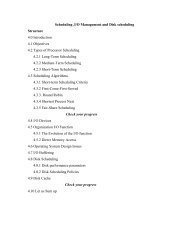
<strong>STRUCTURE</strong><br />
4.0 Objectives<br />
4.1 Introduction<br />
<strong>UNIT</strong>-4: <strong>PARALLEL</strong> <strong>COMPUTER</strong> <strong>MODELS</strong><br />
4.2 Parallel Computer Models<br />
4.2.1 Flynn’s Classification<br />
4.2.2 Parallel and Vector Computers<br />
4.2.3 System Attributes to Performance<br />
4.2.4 Multiprocessors and Multicomputers<br />
4.2.4.1 Shared-Memory Multiprocessors<br />
4.2.4.2 Distributed-Memory Multicomputers<br />
4.2.5 Multivector and SIMDComputers<br />
4.2.5.1 Vector Super Computers<br />
4.2.5.2 SIMD Computers<br />
4.2.6 PRAM and VLSI Models<br />
4.2.6.1 Parallel Random-Access Mach<strong>in</strong>es<br />
4.2.6.2 VLSI Complexity Model<br />
Check Your Progress<br />
4.3 Summary<br />
4.4 Glossary<br />
4.5 References<br />
4.6 Answers to Check Your progress Questions
4.0 OBJECTIVES<br />
After go<strong>in</strong>g through this unit, you will be able to<br />
• describe the Flynn’s classification<br />
• describe parallel and vector computers<br />
• expla<strong>in</strong> system attributes to performance<br />
• dist<strong>in</strong>guish between implicit and explicit parallelism<br />
• expla<strong>in</strong> multiprocessors and multicomputers<br />
• expla<strong>in</strong> multivector and SIMD computers<br />
• describe the PRAM and VLSI models<br />
4.1 INTRODUCTION<br />
Parallel process<strong>in</strong>g has emerged as a key enabl<strong>in</strong>g technology <strong>in</strong> modern computers,<br />
driven by the ever-<strong>in</strong>creas<strong>in</strong>g demand for higher performance, lower costs, and susta<strong>in</strong>ed<br />
productivity <strong>in</strong> real-life applications. Concurrent events are tak<strong>in</strong>g place <strong>in</strong> today’s highperformance<br />
computers due to the common practice of multiprogramm<strong>in</strong>g,<br />
multiprocess<strong>in</strong>g, or multicomput<strong>in</strong>g.<br />
3.2 <strong>PARALLEL</strong> <strong>COMPUTER</strong> <strong>MODELS</strong><br />
Parallelism appears <strong>in</strong> various forms, such as look ahead, pipel<strong>in</strong><strong>in</strong>g vectorization<br />
concurrency, simultaneity, data parallelism, partition<strong>in</strong>g, <strong>in</strong>terleav<strong>in</strong>g, overlapp<strong>in</strong>g,<br />
multiplicity, replication, time shar<strong>in</strong>g, space shar<strong>in</strong>g, multitask<strong>in</strong>g, multiprogramm<strong>in</strong>g,<br />
multithread<strong>in</strong>g, and distributed comput<strong>in</strong>g at different process<strong>in</strong>g levels.<br />
4.2.1Flynn’s Classification<br />
Michael Flynn <strong>in</strong>troduced a classification of various computer architectures based on<br />
notions of <strong>in</strong>struction and data streams. As illustrated <strong>in</strong> the Figure 4.1 conventional<br />
sequential mach<strong>in</strong>es are called SISD Computers. Vector are equipped with scalar and<br />
vector hardware or appear as SIMD mach<strong>in</strong>es. Parallel computers are reserved for MIMD<br />
mach<strong>in</strong>es. An MISD mach<strong>in</strong>es are modeled. The same data stream flows through a l<strong>in</strong>ear<br />
array of processors execut<strong>in</strong>g different <strong>in</strong>struction streams. This architecture is also<br />
known as systolic arrays for pipel<strong>in</strong>ed execution of specific algorithms.<br />
(a) SISD uniprocessor architecture
(b) SIMD architecture (with distributed memory)<br />
(c) MIMD architecture (with shared memory)<br />
(d) MISD architecture (systolic array)<br />
Figure 4.1 Flynn Classification of Computer Architecture
4.2.2 Parallel/Vector Computers<br />
Intr<strong>in</strong>sic parallel computers are those that execute programs <strong>in</strong> MIMD mode. There are<br />
two major classes of parallel computers, namely shared-memory multiprocessors and<br />
message-pass<strong>in</strong>g multicomputers. The major dist<strong>in</strong>ction between multprocessors and<br />
multicomputers lies <strong>in</strong> memory shar<strong>in</strong>g and the mechanisms used for <strong>in</strong>terprocesssor<br />
communication.<br />
The processors <strong>in</strong> a multiprocessor system communicate with each other through shared<br />
variables <strong>in</strong> a common memory. Each computer node <strong>in</strong> a multicomputer system has a<br />
local memory, unshared with other nodes. Inter processor communication is done<br />
through message pass<strong>in</strong>g among the nodes.<br />
Explicit vector <strong>in</strong>structions were <strong>in</strong>troduced with the appearance of vector processors. A<br />
vector processor is equipped with multiple vector pipel<strong>in</strong>es that can be concurrently used<br />
under hardware or firmware control. There are two families of pipel<strong>in</strong>ed vector<br />
processors.<br />
Memory-to-memory architecture supports the pipel<strong>in</strong>ed flow of vector operands directly<br />
from the memory to pipel<strong>in</strong>es and then back to the memory. Register-to-register<br />
architecture uses vector registers to <strong>in</strong>terface between the memory and functional<br />
pipel<strong>in</strong>es.<br />
4.2.3 System Attributes to Performance<br />
The ideal performance of a computer system demands a perfect match between mach<strong>in</strong>e<br />
capability and program behavior. Mach<strong>in</strong>e capability can be enhanced with better<br />
hardware technology architectural features, and efficient resources management.<br />
However, program behavior is difficult to predict due to its heavy dependence on<br />
application and run-time conditions.<br />
There are also many others factors affect<strong>in</strong>g programs behavior, <strong>in</strong>clud<strong>in</strong>g algorithm<br />
design, data structures, language efficiency, programmer skill, and compiler technology.<br />
It is impossible to achieve a perfect match between hardware and software by merely<br />
improv<strong>in</strong>g only a few factors without touch<strong>in</strong>g other factors.<br />
Besides, mach<strong>in</strong>e performance may vary from program to program. This makes peak<br />
performance an impossible target to achieve <strong>in</strong> real-life applications. On the other hand, a<br />
mach<strong>in</strong>e cannot be said to have an average performance either. All performance <strong>in</strong>dices<br />
or benchmark<strong>in</strong>g results must be tied to a program mix. For this reason, the performance<br />
should be described as range or as a harmonic distribution.<br />
Clock Rate and CPI<br />
The CPU (or simply the processor) of today’s digital computer is driven by a clock with<br />
a constant cycle time (T <strong>in</strong> nanoseconds). The <strong>in</strong>verse of the cycle time is the clock rate
(f=1/T <strong>in</strong> megahertz). The size of a program is determ<strong>in</strong>ed by its <strong>in</strong>struction count(Ic), <strong>in</strong><br />
terms of the number of mach<strong>in</strong>e <strong>in</strong>structions to be executed <strong>in</strong> the program. Different<br />
mach<strong>in</strong>e <strong>in</strong>structions may require different numbers of clock cycles to execute.<br />
Therefore, the cycles per <strong>in</strong>struction (CPI) becomes an important parameter for<br />
measur<strong>in</strong>g the time needed to execute each <strong>in</strong>struction.<br />
For a given <strong>in</strong>struction set, we can calculate an average CPI over all <strong>in</strong>struction types,<br />
provided we know their frequencies of appearance <strong>in</strong> the program. An accurate estimate<br />
of the average CPI requires a large amount of program code to be traced over a long<br />
period of time. Unless specifically focus<strong>in</strong>g on a s<strong>in</strong>gle <strong>in</strong>struction type, we simply use<br />
the term CPI to mean the average value with respect to a given <strong>in</strong>struction set and a given<br />
program mix.<br />
Performance Factors:<br />
Let Ic be the number of <strong>in</strong>structions <strong>in</strong> a given program, or the <strong>in</strong>struction count. The<br />
CPU time (T <strong>in</strong> seconds/program) needed to execute the program is estimated by f<strong>in</strong>d<strong>in</strong>g<br />
the product of three contribut<strong>in</strong>g factors:<br />
T=Ic x CPI x τ. (4.1)<br />
The execution of an <strong>in</strong>struction requires go<strong>in</strong>g through a cycle of events <strong>in</strong>volv<strong>in</strong>g the<br />
<strong>in</strong>struction fetch, decode, operand(s) fetch, execution, and store results. In this cycle,<br />
only the <strong>in</strong>struction decodes and execution phases are carried out <strong>in</strong> the CPU. The<br />
rema<strong>in</strong><strong>in</strong>g three operations may be required to access the memory. We def<strong>in</strong>e a memory<br />
cycle is k times the processor cycle T. The value of k depends on the speed of the<br />
memory technology and processor-memory <strong>in</strong>terconnection scheme used.<br />
The CPI of an <strong>in</strong>struction type can be divided <strong>in</strong>to two component terms<br />
correspond<strong>in</strong>g to the total processor cycles and memory cycles needed to complete the<br />
execution of the <strong>in</strong>struction. Depend<strong>in</strong>g on the <strong>in</strong>struction type, the complete <strong>in</strong>struction<br />
cycle may <strong>in</strong>volve to four memory references (one for <strong>in</strong>struction fetch, two for operand<br />
fetch, and one for store results). Therefore we can rewrite Eq. 4.1 as follows:<br />
T=Ic x (p +m x k) x τ. (4.2)<br />
Where p is the number of processor cycles needed for the <strong>in</strong>struction decode and<br />
execution, m is the number of memory references needed, k is the ratio between memory<br />
cycle and processor cycle Ic is the <strong>in</strong>struction count, and T is the processor cycle time.<br />
Equation 4.2 can be further ref<strong>in</strong>ed once the CPI components (p,m,k) are weighted over<br />
the entire <strong>in</strong>struction set.
System Attributes:<br />
The above five performance factors (Ic,p,m,k, τ) are <strong>in</strong>fluenced by four system attributes:<br />
They are <strong>in</strong>struction-set architecture, compiler technology, CPU implementation and<br />
control, and cache and memory hierarchy.<br />
The <strong>in</strong>struction-set architecture affects the program length (Ic) and processor cycle<br />
needed (p). The compiler technology affects the program length (Ic), p, and the memory<br />
reference count (m). The CPU implementation and control determ<strong>in</strong>e the total processor<br />
time (p.τ) needed. F<strong>in</strong>ally, the memory technology and hierarchy design affect the<br />
memory access latency (k.τ). The above CPU time can be used as a basis <strong>in</strong> estimat<strong>in</strong>g<br />
the execution of a processor.<br />
Mips Rate:<br />
Let C be the total number of clock cycles needed to execute a given program. Then the<br />
CPU time can be estimated as T=C x τ =C/F. Furthermore, CPI=C/Ic and T=Ic x CPI x τ<br />
=Ic x CPI/f. the processor speed is often measured <strong>in</strong> terms of million <strong>in</strong>struction per<br />
second(MIPS). We simply call it the MIPS rate of a given processor. It should be<br />
emphasized that the MIPS rate varies with respect to a number of factors, <strong>in</strong>clud<strong>in</strong>g the<br />
clock rate (f), the <strong>in</strong>struction count (Ic), and the CPI of a given mach<strong>in</strong>e, as def<strong>in</strong>ed<br />
below:<br />
MIPS rate = IC / (T x 10 6 ) = f / (CPI x 10 6 ) = (f x Ic) / (C x 10 6 ) (4.3)<br />
Based on Eq. 4.3., the CPU time <strong>in</strong> Eq. 4.2 can be written as T=Ic x 10 -6 /MIPS. Based on<br />
the above derived expressions, we conclude by <strong>in</strong>dicat<strong>in</strong>g the fact that the MIPS rate of a<br />
given computer is directly proportional to the clock rate and <strong>in</strong>versely proportional to the<br />
CPI. All four system attributes, <strong>in</strong>struction set, compiler, processor, and memory<br />
technologies, affect the MIPS rate, which varies also from program to program.<br />
Throughput Rate:<br />
Another important concept is related to how many programs a system can execute per<br />
unit time, called the system throughput Ws (<strong>in</strong> programs/second). In a multiprogrammed<br />
system, the system throughput is often lower than the CPU throughput Wp def<strong>in</strong>ed by:<br />
Wp=f/Ic x CPI (4.4)<br />
The CPU throughput is a measure of how many programs can be executed per Ws
Programm<strong>in</strong>g Environments:<br />
The programmability of a computer depends on the programm<strong>in</strong>g environment<br />
provided to the users. Most computer environments are not user-friendly. In fact, the<br />
marketability of any new computer system depends on the creation of a user-friendly<br />
environment <strong>in</strong> which programm<strong>in</strong>g becomes a joyful undertak<strong>in</strong>g rather than a nuisance.<br />
We briefly <strong>in</strong>troduce below the environmental features desired <strong>in</strong> modern computers.<br />
Conventional uniprocessor computers are programmed <strong>in</strong> a sequential environment <strong>in</strong><br />
which <strong>in</strong>structions are executed one after another <strong>in</strong> a sequential manner. In fact, the<br />
orig<strong>in</strong>al UNIX/OS kernel was designed to respond to one system call from the user<br />
process at a time. Successive system calls must be serialized through the kernel.<br />
Most exist<strong>in</strong>g compilers are designed to generate sequential object codes to run on a<br />
sequential computer. In other words, conventional computers are be<strong>in</strong>g used <strong>in</strong> a<br />
sequential programm<strong>in</strong>g environment us<strong>in</strong>g languages, compilers, and operat<strong>in</strong>g systems<br />
all developed for a uniprocessor computer, desires a parallel environment where<br />
parallelism is automatically exploited. Language extensions or new constructs must be<br />
developed to specify parallelism or to facilitate easy detection of parallelism at various<br />
granularity levels by more <strong>in</strong>telligent compilers.<br />
Implicit Parallelism<br />
An implicit approach uses a conventional language, such as C, FORTRAN, Lisp, or<br />
Pascal, to write the source program. The sequentially coded source program is translated<br />
<strong>in</strong>to parallel object code by a paralleliz<strong>in</strong>g compiler. As illustrated <strong>in</strong> Figure 4.2, this<br />
compiler must be able to detect parallelism and assign target mach<strong>in</strong>e resources. This<br />
compiler approach has been applied <strong>in</strong> programm<strong>in</strong>g shared-memory multiprocessors.<br />
With parallelism be<strong>in</strong>g implicit, success relies heavily on the “<strong>in</strong>telligence” of a<br />
paralleliz<strong>in</strong>g compiler. This approach requires less effort on the part of the programmer.
(a) Implicit parallelism (b) Explicit parallelism<br />
Explicit Parallelism:<br />
Figure 4.2<br />
The second approach requires more effort by the programmer to develop a source<br />
program us<strong>in</strong>g parallel dialects of C, FORTRAN, Lisp, or Pascal. Parallelism is<br />
explicitly specified <strong>in</strong> the user programs. This will significantly reduce the burden on the<br />
compiler to detect parallelism. Instead, the compiler needs to preserve parallelism and,<br />
where possible, assigns target mach<strong>in</strong>e resources. Charles Seitz of California Institute of<br />
Technology and William Dally of Massachusetts Institute of Technology adopted this<br />
explicit approach <strong>in</strong> multicomputer development.<br />
Special software tools are needed to make an environment friendlier to user groups.<br />
Some of the tools are parallel extensions of conventional high-level languages. Others<br />
are <strong>in</strong>tegrated environments which <strong>in</strong>clude tools provid<strong>in</strong>g different levels of program<br />
abstraction, validation, test<strong>in</strong>g, debugg<strong>in</strong>g, and tun<strong>in</strong>g; performance prediction and<br />
monitor<strong>in</strong>g; and visualization support to aid program development, performance<br />
measurement, and graphics display and animation of computer results.
4.2.4 Multiprocessors and Multicomputers<br />
Two categories of parallel computers are architecturally modeled below. These physical<br />
models are dist<strong>in</strong>guished by hav<strong>in</strong>g a shared common memory or unshared distributed<br />
memories.<br />
4.2.4.1 Shared-Memory Multiprocessors<br />
We describe below three shared-memory multiprocessor models: the uniform memoryaccess<br />
(UMA) model, the nonuniform-memory-access(NUMA) model, and the cacheonly<br />
memory architecture(COMA) model. These models differ <strong>in</strong> how the memory and<br />
peripheral resources are shared or distributed.<br />
The UMA Model<br />
In a UMA multiprocessor model (Figure 4.3) the physical memory is uniformly shared by<br />
all the processors. All processors have equal access time to all memory words, which is<br />
why it is called uniform memory access. Each processor may use a private cache.<br />
Peripherals are also shared <strong>in</strong> some fashion.<br />
Multiprocessors are called tightly coupled systems due to the high degree of resource<br />
shar<strong>in</strong>g. The system <strong>in</strong>terconnect takes the form of a common bus , a crossbar switch or a<br />
multistage network.<br />
Most computer manufacturers have multiprocessor extensions of their uniprocessor<br />
product l<strong>in</strong>e. The UMA model is suitable for general purpose and time shar<strong>in</strong>g<br />
applications by multiple users. It can be used to speed up the execution of a s<strong>in</strong>gle large<br />
program <strong>in</strong> time-critical applications. To coord<strong>in</strong>ate parallel events, synchronization and<br />
communication among processors are done through us<strong>in</strong>g shared variables <strong>in</strong> the<br />
common memory.<br />
When all processors have equal access to all peripheral devices, the system is called a<br />
symmetric multiprocessor. In this case, all the processors are equally capable of runn<strong>in</strong>g<br />
the executive programs, such as the OS kernel and I/O service rout<strong>in</strong>es.<br />
In an asymmetric multiprocessor, only one or a subset of processors are executive<br />
capable. An executive or a master processor can execute the operat<strong>in</strong>g system and handle<br />
I/O. The rema<strong>in</strong><strong>in</strong>g processors have no I/O capability and thus are called attached<br />
processors (APs). Attached processors execute user codes under the supervision of the<br />
master processor. In both multiprocessor and attached processor configurations,<br />
memory shar<strong>in</strong>g among master and attached processors is still <strong>in</strong> place.
Figure 4.3 The UMA multiprocessor model<br />
Approximated performance of a multiprocessor<br />
This example exposes the reader to parallel program execution on a shared memory<br />
multiprocessor system. Consider the follow<strong>in</strong>g Fortran program written for sequential<br />
execution on a uniprocessor system. All the arrays , A(I), B(I), and C(I), are assumed to<br />
have N elements.<br />
L1: Do 10 I=1, N<br />
L2: A(I) = B(I) + C(I).<br />
L3: 10 Cont<strong>in</strong>ue<br />
L4: SUM = 0.<br />
L5: Do 20 J = 1, N<br />
L6: SUM = SUM + A(J).<br />
L7: 20 Cont<strong>in</strong>ue<br />
Suppose each l<strong>in</strong>e of code L2, L4, and L6 takes 1 mach<strong>in</strong>e cycle to execute. The time<br />
required to execute the program control statements L1, L3, L5, and L7 is ignored to<br />
simplify the analysis. Assume that k cycles are needed for each <strong>in</strong>terprocessor<br />
communication operation via the shared memory.<br />
Initially, all arrays are assumed already loaded <strong>in</strong> the ma<strong>in</strong> memory and the short<br />
program fragment already loaded <strong>in</strong> the <strong>in</strong>struction cache. In other words <strong>in</strong>struction<br />
fetch and data load<strong>in</strong>g overhead is ignored. Also, we ignore bus contention or memory<br />
access conflicts problems. In this way, we can concentrate on the analysis of CPU<br />
demand.
The above program can be executed on a sequential mach<strong>in</strong>e <strong>in</strong> 2N cycles under the<br />
above assumption. N cycles are needed to execute the N <strong>in</strong>dependent iterations <strong>in</strong> the I<br />
loop. Similarly, N cycles are needed for the J loop, which conta<strong>in</strong>s N recursive iterations.<br />
To execute the program on an M-processor system, we partition the loop<strong>in</strong>g operations<br />
<strong>in</strong>to M sections with L= N/M elements per section. In the follow<strong>in</strong>g parallel code, Doall<br />
declares that all M sections be executed by M processors <strong>in</strong> parallel.<br />
Doall K=1,M<br />
Do 10 I = L(K-1) + 1, KL<br />
A(I) = B(I) + C(I).<br />
10 Cont<strong>in</strong>ue<br />
SUM(K) = 0<br />
Do 20 J = 1, L<br />
SUM(K) = SUM(K) + A(L(K – 1) + J)<br />
20 Cont<strong>in</strong>ue<br />
Endall<br />
For M-way parallel execution, the sectioned I loop can be done <strong>in</strong> L cycles. The sectioned<br />
J loop produces M partial sums <strong>in</strong> L cycles. Thus 2L cycles are consumed to produce all<br />
M partial sums. Still, we need to merge these M partial sums to produce the f<strong>in</strong>al sum of<br />
N elements.<br />
The NUMA Model:<br />
A NUMA multiprocessor is a shared-memory system <strong>in</strong> which the access time varies<br />
with the location of the memory word. Two NUMA mach<strong>in</strong>e models are depicted <strong>in</strong> the<br />
Figure 4.4<br />
(a) Shared local memories
(b) A hierarchical cluster model<br />
Figure 4.4<br />
The shared memory is physically distributed to all processors, called local memories.<br />
The collection of all local memories forms a global address space accessible by all<br />
processors.<br />
It is faster to access a local memory with a local processor. The access of remote<br />
memory attached to other processors takes longer due to the added delay through the<br />
<strong>in</strong>terconnection network. The BBN TC-2000 Butterfly multiprocessor assumes the<br />
configuration.<br />
Besides distributed memories, globally shared memory can be added to a multiprocessor<br />
system. In this case, there are three memory-access patterns: The fastest is local memory<br />
access. The next is global memory access. The slowest is access of remote memory. As a<br />
mater of fact, the models can be easily modified to allow a mixture of shared memory<br />
and private memory with pre specified access rights.<br />
A hierarchically structured multiprocessor is modeled. The processors are divided <strong>in</strong>to<br />
several clusters. Each cluster is itself an UMA or a NUMA multiprocessor. The clusters<br />
are connected to global shared-memory modules. The entire system is considered a<br />
NUMA multiprocessor. All processors belong<strong>in</strong>g to the same cluster are allowed to<br />
uniformly access the cluster shared-memory modules.
All clusters have equal access to the global memory. However, the access time to the<br />
cluster memory is shorter than that to the global memory. One can specify the access<br />
right among <strong>in</strong>tercluster memories <strong>in</strong> various ways. The Cedar multiprocessor, built at<br />
the University of Ill<strong>in</strong>ois, assumes such a structure <strong>in</strong> which each cluster is an Alliant<br />
FX/80 multiprocessor.<br />
The COMA Model:<br />
A multiprocessor us<strong>in</strong>g cache-only memory assumes the COMA model. The COMA<br />
model (Figure 4.5) is a special case of a NUMA mach<strong>in</strong>e, <strong>in</strong> which the distributed ma<strong>in</strong><br />
memories are converted to caches. There is no memory hierarchy at each processor node.<br />
All the caches form a global address space. Remote cache access is assisted by the<br />
distributed cache directories. Depend<strong>in</strong>g on the <strong>in</strong>terconnection network used, sometimes<br />
hierarchical directories may be used to help locate copies of cache blocks. Initial data<br />
placement is not critical because data will eventually migrate to where it will be used.<br />
Figure 4.5 The COMA model of a multiprocessor<br />
Besides the UMA, NUMA, and COMA models specified above, other variations exist for<br />
mutliprocessors. For example, a cache-coherent non-uniform memory access (CC-<br />
NUMA) model can be specified with distributed shared memory and cache directories.<br />
One can also <strong>in</strong>sist on a cache-coherent COMA mach<strong>in</strong>e <strong>in</strong> which all cache copies must<br />
be kept consistent.<br />
4.1.4.2 Distributed-Memory Multicomputers<br />
A distributed-memory multicomputer system is modeled <strong>in</strong> Figure 4.6. The system<br />
consists of multiple computers, often called nodes, <strong>in</strong>terconnected by a message-pass<strong>in</strong>g<br />
network. Each node is an autonomous computer consist<strong>in</strong>g of a processor, local memory,<br />
and sometimes attached disks or I/O peripherals.
Figure 4.6 Generic model of a message-pass<strong>in</strong>g multicomputer<br />
The message-pass<strong>in</strong>g network provides po<strong>in</strong>t-to-po<strong>in</strong>t static connections among the<br />
nodes. All local memories are private and are accessible only by local processors. For this<br />
reason, traditional multicomputers have been called no-remote-memory-access<br />
(NORMA) mach<strong>in</strong>es. However, this restriction will gradually be removed <strong>in</strong> future<br />
multicomputers with distributed shared memories. Internode communication is carried<br />
out by pass<strong>in</strong>g messages to the static connection network.<br />
4.2.5 Multivector and SIMD Computers:<br />
We classify supercomputers either as pipel<strong>in</strong>ed vector mach<strong>in</strong>es us<strong>in</strong>g a few powerful<br />
processors equipped with vector hardware, or as SIMD computers emphasiz<strong>in</strong>g massive<br />
data parallelism.<br />
4.2.5.1Vector Supercomputers:<br />
A vector computer is often built on top of a scalar processor. As shown <strong>in</strong> Figure 4.7, the<br />
vector processor is attached to the scalar processor as an optional feature. Program and<br />
data are first loaded <strong>in</strong>to the ma<strong>in</strong> memory through a host computer. All <strong>in</strong>structions are<br />
first decoded by the scalar control unit. If the decoded <strong>in</strong>struction is a scalar operation or<br />
a program control operation, it will be directly executed by the scalar processor us<strong>in</strong>g the<br />
scalar functional pipel<strong>in</strong>es.
If the <strong>in</strong>structions are decoded as a vector operation, it will be sent to the vector control<br />
unit. This control unit will supervise the flow of vector data between the ma<strong>in</strong> memory<br />
and vector functional pipel<strong>in</strong>es. The vector data flow is coord<strong>in</strong>ated by the control unit.<br />
A number of vector functional pipel<strong>in</strong>es may be built <strong>in</strong>to a vector processor.<br />
Vector Processor Model:<br />
The Fig. 4.7 shows a register-to-register architecture. Vector registers are used to hold<br />
the vector operands, <strong>in</strong>termediate and f<strong>in</strong>al vector results. The vector functional pipel<strong>in</strong>es<br />
retrieve operands from and put results <strong>in</strong>to the vector registers. All vector registers are<br />
programmable <strong>in</strong> user <strong>in</strong>structions. Each vector register is equipped with a component<br />
counter which keeps track of the component registers used <strong>in</strong> successive pipel<strong>in</strong>es cycles.<br />
Figure 4.7 The architecture of a vector super computer<br />
The length of each vector register is usually fixed, say, sixty-four 64-bit component<br />
registers <strong>in</strong> a vector register <strong>in</strong> a Cray Series supercomputers. Other mach<strong>in</strong>es, like the<br />
Fujitsu VP2000 Series, use reconfigurable vector registers to dynamically match the<br />
register length with that of the vector operands.<br />
In general, there are fixed numbers of vector registers and functional pipel<strong>in</strong>es <strong>in</strong> a vector<br />
processor. Therefore, both resources must be reserved <strong>in</strong> advance to avoid resource<br />
conflicts between vector operations. A memory-to-memory architecture differs from a
egister-to-register architecture <strong>in</strong> the use of a vector stream unit to replace the vector<br />
registers. Vector operands and results are directly retrieved from the ma<strong>in</strong> memory <strong>in</strong><br />
super words, say, 512 bits as <strong>in</strong> the Cyber 205.<br />
4.2.5.2 SIMD Supercomputers<br />
In Figure 4.1b, we have shown an abstract model of a SIMD computer, hav<strong>in</strong>g a s<strong>in</strong>gle<br />
<strong>in</strong>struction stream over multiple data streams. An operational model of an SIMD<br />
computer is shown <strong>in</strong> Figure 4.8.<br />
SIMD Mach<strong>in</strong>e Model:<br />
An operational model of an SIMD computer is specified by a 5-tuple:<br />
where<br />
M = (4.5)<br />
(1) N is the number of process<strong>in</strong>g elements (PEs) <strong>in</strong> the mach<strong>in</strong>e. For<br />
example, Illiac IV has 64 PEs and the Connection Mach<strong>in</strong>e CM-2 uses<br />
65,536 PEs.<br />
(2) C is the set of <strong>in</strong>structions directly executed by the control unti(CU),<br />
<strong>in</strong>clud<strong>in</strong>g scalar and program flow control <strong>in</strong>structions,<br />
(3) I is the set of <strong>in</strong>structions broadcast by the CU to all PEs for parallel<br />
execution. These <strong>in</strong>clude arithmetic, logic, data rout<strong>in</strong>g, mask<strong>in</strong>g, and<br />
other local operations executed by each active PE over data with<strong>in</strong> that<br />
PE.<br />
(4) M is the set of mask<strong>in</strong>g schemes, where each mask partitions the set<br />
of PEs <strong>in</strong>to enabled and disabled subsets.<br />
(5) R is the set of data-rout<strong>in</strong>g functions, specify<strong>in</strong>g various patterns to be<br />
set up <strong>in</strong> the <strong>in</strong>terconnection network for <strong>in</strong>ter-PE communications.<br />
Figure 4.8 Operational model of SIMD computer
4.2.6 PRAM and VLSI Models<br />
Theoretical models of parallel computers are abstracted from the physical models studied<br />
<strong>in</strong> previous sections. These models are often used by algorithm designers and VLSI<br />
device/chip developers. The ideal models provide a convenient framework for develop<strong>in</strong>g<br />
parallel algorithms without worry<strong>in</strong>g about the implementation details or physical<br />
constra<strong>in</strong>ts.<br />
The models can be applied to obta<strong>in</strong> theoretical performance bounds on parallel<br />
computers or to estimate VLSI complexity on chip area and execution time before the<br />
chip is fabricated. The abstract models are also useful <strong>in</strong> scalability and programmability<br />
analysis, when real mach<strong>in</strong>es are compared with an idealized parallel mach<strong>in</strong>e without<br />
worry<strong>in</strong>g about communication overhead among process<strong>in</strong>g nodes.<br />
4.2.6.1 Parallel Random-Access Mach<strong>in</strong>es:<br />
Theoretical models of parallel computers are presented below. We def<strong>in</strong>e first the time<br />
and space complexities. Computational tractability is reviewed for solv<strong>in</strong>g difficult<br />
problems on computers. Then we <strong>in</strong>troduce the random-access mach<strong>in</strong>e (RAM), parallel<br />
random-access mach<strong>in</strong>e (PRAM), and variants of PRAMs. These complexity models<br />
facilitate the study of asymptotic behavior of algorithms implementable on parallel<br />
computers.<br />
Time and Space Complexities:<br />
The complexity of an algorithm for solv<strong>in</strong>g a problem of size s on a computer is<br />
determ<strong>in</strong>ed by the execution time and the storage space required. The time complexity is a<br />
function of the problem size. The time complexity function <strong>in</strong> order notation is the<br />
asymptotic time complexity of the algorithm. Usually, the worst-case time complexity is<br />
considered. For example, a time complexity g(s) is said to be O(f(s)), read “order f(s)”, if<br />
there exist positive constants c and s0 such that g(s) s0.<br />
The space complexity can be similarly def<strong>in</strong>ed as a function of the problem size s. The<br />
asymptotic space complexity refers to the data storage of large problems. Note that the<br />
program (code) storage requirement and the storage for <strong>in</strong>put data are not considered <strong>in</strong><br />
this.<br />
The time complexity of a serial algorithm is simply called serial complexity. The time<br />
complexity of a parallel algorithm is called parallel complexity. Intuitively, the parallel<br />
complexity should be lower than the serial complexity, at least asymptotically. We<br />
consider only determ<strong>in</strong>istic algorithms, <strong>in</strong> which every operational step is uniquely<br />
def<strong>in</strong>ed <strong>in</strong> agreement with the way programs are executed on real computers.
A nondeterm<strong>in</strong>istic algorithm conta<strong>in</strong>s operations result<strong>in</strong>g <strong>in</strong> one outcome <strong>in</strong> a set of<br />
possible outcomes. There exist no real computers that can execute nondeterm<strong>in</strong>istic<br />
algorithms.<br />
PRAM Models<br />
Conventional uniprocessor computers have been modeled as random access mach<strong>in</strong>es by<br />
Sheperdson and Sturgis. A parallel random-access mach<strong>in</strong>e (PRAM) model has been<br />
developed by Fortune and Wyllie for model<strong>in</strong>g idealized parallel computers with zero<br />
synchronization or memory access overhead. This PRAM model will be used for parallel<br />
algorithm development and for scalability and complexity analysis.<br />
Figure 4.9 PRAM model of a multiprocessor system<br />
An n-processor PRAM (Figure 4.9) has a globally addressable memory. The shared<br />
memory can be distributed among the processors or centralized <strong>in</strong> one place. The n<br />
processors operate on a synchronized read-memory, compute, and write-memory cycle.<br />
With shared memory, the model must specify how concurrent read and concurrent write<br />
of memory are handled. Four memory-update options are possible.<br />
• Exclusive read (ER) – This allows at most one processor to read from any<br />
memory location <strong>in</strong> each cycle, a rather restrictive policy.<br />
• Concurrent read (CR) – This allows multiple processors to read the same<br />
<strong>in</strong>formation from the same memory cell <strong>in</strong> the same cycle.<br />
• Concurrent write (CW) – this allows simultaneous writes to the same memory<br />
location. In order to avoid confusion, some policy must be set up to resolve the<br />
write conflicts.
Various comb<strong>in</strong>ations of the above options lead to several variants of the PRAM model<br />
as specified below. S<strong>in</strong>ce CR does not create a conflict problem, variants differ ma<strong>in</strong>ly <strong>in</strong><br />
how they handle the CW conflicts.<br />
PRAM Variants:<br />
Described below are four variants of the PRAM model, depend<strong>in</strong>g on how the memory<br />
reads and writes are handled.<br />
(1) The EREW-PRAM model – This model forbids more than one processor from<br />
read<strong>in</strong>g or writ<strong>in</strong>g the same memory cell simultaneously. This is the most<br />
restrictive PRAM model proposed.<br />
(2) The CREW-PRAM model – The write conflicts are avoided by mutual<br />
exclusion. Concurrent reads to the same memory location are allowed.<br />
(3) The ERCW-PRAM model – This allows exclusive read or concurrent writes<br />
to the same memory location.<br />
(4) The CRCW-PRAM model – This model allows either concurrent reads or<br />
concurrent writes at the same time. The conflict<strong>in</strong>g writes are resolved by one<br />
of the follow<strong>in</strong>g four polices :<br />
4.2.6.2 VLSI Complexity Model:<br />
Common – All simultaneous writes store the same value to the<br />
hot-spot memory location.<br />
Arbitrary – Any one of the values written may rema<strong>in</strong>; the others<br />
are ignored.<br />
M<strong>in</strong>imum – The value written by the processor with the m<strong>in</strong>imum<br />
<strong>in</strong>dex will rema<strong>in</strong>.<br />
Priority – The values be<strong>in</strong>g written are comb<strong>in</strong>ed us<strong>in</strong>g some<br />
associative functions, such as summation or maximum.<br />
Parallel computers rely on the use of VLSI chips to fabricate the major components such<br />
as processor arrays, memory arrays, and large-scale switch<strong>in</strong>g networks. An AT power 2<br />
model for two-dimensional VLSI chips is presented below, based on the work of Clark<br />
Thomson. Three lower bounds on VLSI circuit are <strong>in</strong>terpreted by Jeffrey Ullaman. The<br />
bounds are obta<strong>in</strong>ed by sett<strong>in</strong>g limits on memory, I/O, and communication for<br />
implement<strong>in</strong>g parallel algorithms with VLSI chips.
The AT 2 Model:<br />
Let A be the chip area and T be the latency for complet<strong>in</strong>g a given computation us<strong>in</strong>g a<br />
VLSI circuit chip. Let s by the problem size <strong>in</strong>volved <strong>in</strong> the computation. Thompson<br />
stated <strong>in</strong> his doctoral thesis that for certa<strong>in</strong> computations, there exists a lower bound f(s)<br />
such that<br />
A x T 2 >=O (f(s)) (4.6)<br />
The chip area A is a measure of the chip’s complexity. The latency T is the time required<br />
from when <strong>in</strong>puts are applied until all outputs are produced for a s<strong>in</strong>gle problem <strong>in</strong>stance.<br />
The chip is represented by the base area <strong>in</strong> the two horizontal dimensions. The vertical<br />
dimension corresponds to time. Therefore, the three-dimensional solid represents the<br />
history of the computation performed by the chip.<br />
Memory Bound Chip Area A:<br />
There are many computations which are memory-bound, due to the need to process large<br />
data sets. To implement this type of computation <strong>in</strong> silicon, one is limited by how densely<br />
<strong>in</strong>formation (bit cells) can be placed on the chip. As depicted <strong>in</strong> Figure 4.10a, the<br />
memory requirement of a computation sets a lower bound on the chip area A.<br />
The amount of <strong>in</strong>formation processed by the chip can be visualized as <strong>in</strong>formation flow<br />
upward across the chip area. Each bit can flow through a unit area of the horizontal chip<br />
slice. Thus, the chip area bounds the amount of memory bits stored on the chip.<br />
(a) Memory-limited bound on chip area A and I/O-limited bound on chip<br />
history represented by the volume AT
__<br />
(b)Communication-limited bound on the bisection √A T<br />
I/O Bound on Volume AT:<br />
Figure 4.10<br />
The volume of the rectangular cube is represented by the product AT. As <strong>in</strong>formation<br />
flows through the chip for a period of time T, the number of <strong>in</strong>put bits cannot exceed the<br />
volume. This provides an I/O-limited lower bound on the product AT, as demonstrated.<br />
The area A corresponds to data <strong>in</strong>to and out of the entire surface of the silicon chip. This<br />
area measure sets the maximum I/O limit rather than us<strong>in</strong>g peripheral I/O pads as seen <strong>in</strong><br />
conventional chips. The height T of the volume can be visualized as a number of<br />
snapshots on the chip, as comput<strong>in</strong>g time elapses. The volume represents the amount of<br />
<strong>in</strong>formation flow<strong>in</strong>g through the chip dur<strong>in</strong>g the entire course of the computation.<br />
__<br />
Bisection Communication Bound, √A T:<br />
__<br />
It depicts a communication limited lower bound on the bisection area √AT. The bisection<br />
is represented by the vertical slice cutt<strong>in</strong>g across the shorter dimension of the chip area.<br />
The distance of this dimension is at most square root A for a square chip. The height of<br />
the cross section is T.<br />
The bisection area represents the maximum amount of <strong>in</strong>formation exchange between the<br />
two halves of the chip circuit dur<strong>in</strong>g the time period T. The cross-section area √AT limits
the communication bandwidth of a computation. VLSI complexity theoreticians have<br />
used the square of this measure AT 2 , as the lower bound.<br />
Charles Seitz has given another <strong>in</strong>terpretation of the AT 2 result. He considers the areatime<br />
product AT the cost of a computation, which can be expected to vary as 1/T. This<br />
implies that the cost of computation for a two-dimensional chip decreases with the<br />
execution time allowed.<br />
When three-dimensional (multilayer) silicon chips are used, Seitz asserted that the cost of<br />
computation, as limited by volume-time product, would vary as 1/√T. This is due to that<br />
the bisection will vary as (AT) 2/3 for 3-D chips <strong>in</strong>stead of as square AT for 2-D chips.<br />
CHECK YOUR PROGRESS<br />
1. Conventional sequential mach<strong>in</strong>es are called<br />
(a) SISD (b) SIMD (c) MISD (d) MIMD<br />
2. MISD architecture is also known as<br />
(a) vector computer (b) systolic array (c) parallel computer (d) sequential structure<br />
3.The CPU time needed to execute the program is<br />
(a) T = Ic x CPI x τ (b) T = Ic x CPI / τ (c) T = Ic x τ / CPI (d) T = Ic x CPI x τ + k<br />
4. Processor hav<strong>in</strong>g equal access to all peripheral devices is called<br />
(a) symmetric processor (b) asymmetric processor<br />
(c) attached processor (d) associative processor<br />
5. The PRAM model which allows either concurrent read or concurrent write at the same<br />
time is called<br />
(a) EREW model (b) CREW model(c) ERCW model (d) CRCW model<br />
4.3 SUMMARY<br />
• Flynn classifies the computers <strong>in</strong>to four categories of computer architectures<br />
• Intr<strong>in</strong>sic parallel computers are those that execute programs <strong>in</strong> MIMD mode<br />
• Conventional sequential computers are called SISD<br />
• Vector computer equipped with scalar and vector hardware is called SIMD<br />
• Parallel computers are reserved for MIMD<br />
• MISD is systolic architecture<br />
• In a UMA multiprocessor model the physical memory is uniformly shared by all<br />
the processors<br />
• NUMA multiprocessor is a shared-memory system <strong>in</strong> which the access time vary<br />
with the location of the memory word
• In COMA model remote cache access is assisted by the distributed cache<br />
directories<br />
• Variants of PRAM are EREW, CREW, ERCW, CRCW<br />
• Parallel computers rely on the use of VLSI chip<br />
4.4 GLOSSARY<br />
COMA : Cache-only memory architecture<br />
MIMD : Multiple <strong>in</strong>struction multiple data stream<br />
MIPS : Million <strong>in</strong>structions per second<br />
MISD : Multiple <strong>in</strong>struction s<strong>in</strong>gle data stream<br />
NUMA : Nonuniform memory access<br />
PRAM : Parallel random access mach<strong>in</strong>e<br />
SISD : S<strong>in</strong>gle <strong>in</strong>struction s<strong>in</strong>gle data stream<br />
SIMD : S<strong>in</strong>gle <strong>in</strong>struction multiple data stream<br />
Throughput : A measure of how many programs can be executed per second<br />
UMA : Uniform memory access<br />
4.5 REFERENCE<br />
1. Thomas C Bartee “Computer architecture and logic design” TMH<br />
2. Kai Hwang “Advanced computer architecture: Parallelism, scalability,<br />
programability”, TMH<br />
3. Hamacher, Vranesic, and Zaki “Computer organization” TMH<br />
4. Hayes “Computer architecture and organization”, THH<br />
4.6 ANSWERS TO CHECK YOUR PROGRESS QUESTIONS<br />
1. (a) , 2. (b), 3. (a), 4.(a), 5.(d)