GratinGs: theory and numeric applications - Institut Fresnel

More documents

Recommendations

Info

11.6 Gratings: Theory and Numeric Applications, 2012 which from (A ) leads to (A 1) : − ∂ ∂yi ( ε −1 i j (y)∂H1 ) = ∂yj ( ∂H0 ∂zj )( ∂ ε ∂yi −1 i j (y) ) . We can look at (A 1) as an equation for the unknown H1(x,y), periodic of period Y in y and parametrized by x. Such an equation is solved up to an additive constant. In addition to that, the parameter x is only involved via the factor ∂H0/∂zj. Hence, by linearity, we can write the solution H1(x,y) as follows: H1(x,y) = ∂H0(x) w j (y) , where the two functions w j (y), j = 1,2 are solutions to (A 1) corresponding to ∂H0/∂zj(x), j = 1,2 equal to unity with the other ones being zero, that is solutions to: (A 2) : − ∂ ( ε ∂yi −1 i j (y)∂wk ) ( ∂ = δ jk ε ∂yj ∂yi −1 i j (y) ) , σ 0 i (x,y) = ε −1 i j (y) ( ∂H0 ∂zj + ∂H1 ∂yj ∂zj with wk (y), k = 1,2 periodic functions in y of period Y 2 . Since the functions wk (y) are known, we note that ) = ε −1 i j (y) which can be written as σ i 0 (x,y) = ( ( ∂H0 ∂zj + ∂H0 ∂zk ε −1 ik (y) + ε−1 i j (y)∂wk ) (y) ∂H0(x) . ∂yj ∂zk Lets us now apply the mean to both sides of this equation. We obtain: < σ i 0 ∂H0(x) > (x) = ε−1 hom,ik , ∂zk ∂wk ) (y) , which can be recast as the following homogenized problem: ⎧ 2 ( ⎪⎨ ∂ − ∑ ε (P0) : i,k=1 ∂xi ⎪⎩ −1 ) ∂H0(x) hom,ik = ω ∂xk 2 µ0ε0H0(x) ,in Ω f , ε −1 x hom,ik ( η )∂H0(x) ∂xi ∂yj nk = 0 ,on ∂Ωf , where ε −1 hom,ik denote the coefficients of the homogenized matrix of permittivity given by: ε −1 ∫ ∫ ( 1 hom,ik = | Y | Y ε −1 ik (y) + ε−1 i j (y)∂wk ) (y) dy . (11.4) ∂yj As an illustrative example for this homogenized problem, we consider a microstructured waveguide consisting of a medium with relative permittivity ε = 1.25 with elliptic inclusions (of minor 2 We note that (A 2) are two equations which merely depend upon ε −1 i j (y), that is on the microscopic properties of the periodic medium. The two functions w k (defined up to an additive constant) can be computed once for all, independently of Ω f .
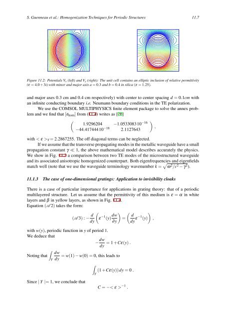
S. Guenneau et al.: Homogenization Techniques for Periodic Structures 11.7 Figure 11.2: Potentials Vx (left) and Vy (right): The unit cell contains an elliptic inclusion of relative permittivity (ε = 4.0 + 3i) with minor and major axis a = 0.3 and b = 0.4 in silica (ε = 1.25). and major axes 0.3 cm and 0.4 cm respectively) with center to center spacing d = 0.1cm with an infinite conducting boundary i.e. Neumann boundary conditions in the TE polarization. We use the COMSOL MULTIPHYSICS finite element package to solve the annex problem and we find that [εhom] from (11.4) writes as [26] ( 1.9296204 −1.053308310−16 −44.41744410−18 ) , 2.1127643 with < ε >Y = 2.2867255. The off diagonal terms can be neglected. If we assume that the transverse propagating modes in the metallic waveguide have a small propagation constant γ ≪ 1, the above mathematical model describes accurately the physics. We show in Fig. 11.3 a comparison between two TE modes of the microstructured waveguide and its associated anisotropic homogenized counterpart. Both eigenfrequencies and eigenfields match well (note that we use the waveguide terminology wavenumber k = √ ω 2 /c 2 − γ 2 ). 11.1.3 The case of one-dimensional gratings: Application to invisibility cloaks There is a case of particular importance for applications in grating theory: that of a periodic multilayered structure. Let us assume that the permittivity of this medium is ε = α in white layers and β in yellow layers, as shown in Fig. 11.4. Equation (A 2) takes the form: (A 3) : − d dy ( ε −1 (y) dw ) ( d = ∂y dy ε−1 ) (y) , with w(y), periodic function in y of period 1. We deduce that − dw = 1 +Cε(y) . dy ∫ Noting that Y dw dy Since | Y |= 1, we conclude that = w(1) − w(0) = 0, this leads to ∫ Y (1 +Cε(y))dy = 0 . C = −< ε > −1 .
Page 1 and 2: GratinGs: theory and numeric applic
Page 3 and 4: Chapter 11: Homogenization Techniqu
Page 5 and 6: Chapter 11 Homogenization Technique
Page 8 and 9: 11.4 Gratings: Theory and Numeric A
Page 12 and 13: 11.8 Gratings: Theory and Numeric A
Page 14 and 15: 11.10 Gratings: Theory and Numeric

GratinGs: theory and numeric applications - Institut Fresnel

Create successful ePaper yourself

Delete template?

Save as template?