GratinGs: theory and numeric applications - Institut Fresnel

More documents

Recommendations

Info

11.12 Gratings: Theory and Numeric Applications, 2012 The subsequent asymptotic development considers small perturbations about the points Γ, X and M so that the boundary conditions of u on the outer boundaries of the cell, namely ∂S1, read, u| ξi=1 = ±u| ξi=−1 and u ,ξi | ξi=1 = ±u ,ξi | ξi=−1, (11.12) where the +,− stand for periodic and anti-periodic conditions respectively: the standing waves occur when these conditions are met. The conditions on ∂S2 are either of Dirichlet or Neumann type. The theory that follows is similar for both boundary condition cases, but the latter one is illustrated herein. Neumann boudary condition on the hole’s surface or equivalently electromagnetic waves in TE polarization yield, which in terms of the two-scales and ui(X,ξξξ ) become ∂u ∂n = u,xini| ∂S2 = 0. (11.13) U 0,ξi ni = 0, (U0 f0,Xi + u 1,ξi )ni = 0, (u1,Xi + u 2,ξi )ni = 0. (11.14) The solution of the leading order equation is by introducing the following separation of variables u0 = f0(X)U0(ξξξ ;Ω0). It is obvious that f0(X), which represents the behaviour of the solution in the long scale, is not set by the leading order equation and the resulting eigenvalue problem is solved on the short-scale for Ω0 and U0 representing the standing wave frequencies and the associated cell’s vibration modes respectively. To solve the first order equation (11.10) we take the integral over the cell of the product of equation (11.10) with U0 minus the product of equation (11.9) with u1/ f0 and this yields Ω1 = 0. It then follows to solve for u1(X,ξξξ ) = f0,Xi (X)U1i (ξξξ ) where the vector U1 is found as in [40]. By invoking a similar solvability condition for the second order equation we obtain a second order PDE for f0(X), Ti j f0,XiXj + Ω2 2 f0 = 0 where, ti j Ti j = ∫ ∫ SU2 0 dS for i, j = 1,2 (11.15) entirely on the long scale with the coefficients Ti j containing all the information of the cell’s dynamical response and the tensor ti j represents dynamical averages of the properties of the medium. For Neumann boundary conditions on ∂S2 its formulation reads, ∫ ∫ tii = U 2 ∫ ∫ 0 dS + (U1i,ξiU0 −U1iU0,ξi )dS for i = 1 or 2, (11.16) S ∫ ∫ ti j = S S (U1 j,ξiU0 −U1 jU0,ξi )dS for i ̸= j. (11.17) Note that there is no summation over repeated indexes for tii. The tensor depends on the boundary conditions of the holes and has a different form if Dirichlet type conditions are applied on ∂S2. The PDE for f0 has several uses, and can be verified by re-creating asymptotically the dispersion curves for a perfect lattice system. One important result of equation (11.15) is its use in the expansion of Ω namely in equation (11.8). In order to obtain Ω2 as a function of the Bloch wavenumbers we use the Bloch boundary conditions on the cell to solve for f0(X) = exp(iκ jXj/η), where κ j = Kj − d j with d j = 0,π/2,−π/2 depending on the location in the Brillouin zone. The asymptotic dispersion relation now reads, Ω ∼ Ω0 + Ti j κiκ j. (11.18) 2Ω0
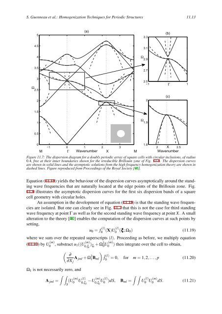
S. Guenneau et al.: Homogenization Techniques for Periodic Structures 11.13 5 4.5 4 3.5 3 Ω 2.5 2 1.5 1 0.5 0 M (a) −1 0 1 2 3 Γ Wavenumber X M 3.3 3.1 Ω 2.9 2.7 (b) 2.5 −1 Γ 1 2 Ω 1.9 1.8 (c) 2 X 2.5 Wavenumber Figure 11.7: The dispersion diagram for a doubly periodic array of square cells with circular inclusions, of radius 0.4, free at their inner boundaries shown for the irreducible Brillouin zone of Fig. 11.6. The dispersion curves are shown in solid lines and the asymptotic solutions from the high frequency homogenization theory are shown in dashed lines. Figure reproduced from Proceedings of the Royal Society [40]. Equation (11.18) yields the behaviour of the dispersion curves asymptotically around the standing wave frequencies that are naturally located at the edge points of the Brillouin zone. Fig. 11.8 illustrates the asymptotic dispersion curves for the first six dispersion bands of a square cell geometry with circular holes. An assumption in the development of equation (11.18) is that the standing wave frequencies are isolated. But one can clearly see in Fig. 11.7 that this is not the case for third standing wave frequency at point Γ as well as for the second standing wave frequency at point X. A small alteration to the theory [40] enables the computation of the dispersion curves at such points by setting, u0 = f (l) 0 (X)U(l) 0 (ξξξ ;Ω0) (11.19) where we sum over the repeated superscripts (l). Proceeding as before, we multiply equation (11.10) by U (m) 0 , substract u1((U (m) 0,ξi ) ξi + Ω2 0 U(m) 0 ) then integrate over the cell to obtain, Ω1 is not necessarily zero, and ∫ ∫ A jml = ( ∂ A jml + Ω ∂Xj 2 ) 1Bml S ˆf (l) 0 (U (m) 0 U(l) 0,ξ j −U(m) 0,ξ j U(l) 0 )dS, Bml = = 0, for m = 1,2,..., p (11.20) ∫ ∫ U (l) 0 U(m) 0 dS. (11.21)
Page 1 and 2: GratinGs: theory and numeric applic
Page 3 and 4: Chapter 11: Homogenization Techniqu
Page 5 and 6: Chapter 11 Homogenization Technique
Page 8 and 9: 11.4 Gratings: Theory and Numeric A
Page 14 and 15: 11.10 Gratings: Theory and Numeric

GratinGs: theory and numeric applications - Institut Fresnel

You also want an ePaper? Increase the reach of your titles

Delete template?

Save as template?