GratinGs: theory and numeric applications - Institut Fresnel

More documents

Recommendations

Info

11.10 Gratings: Theory and Numeric Applications, 2012 Figure 11.5: Propagation of a plane wave of wavelength 7 10 −7 m (red in the visible spectrum) from the left on a multilayered cloak of inner radius R1 = 1.5 10 −8 m and outer radius R2 = 3 10 −8 m, consisting of 20 homogeneous layers of equal thickness and of respective relative permittivities 1680.70,0.25,80.75,0.25,29.39,0.25,16.37,0.25,10.99,0.25,8.18,0.25,6.50,0.25,5.40, 0.25,4.63,0.25,4.06,0.25 in vacuum. Importantly, one layer in two has the same permittivity. 11.2.1 High Frequency Homogenization for Scalar Waves Waves propagating through photonic crystals and metamaterials have proven to show different effects depending on their frequency. The homogenization of a periodic material is not unique. The effective properties of a periodic medium change depending on the vibration modes within its cells. The dispersion diagram structure can be considered to be the identity of such a material and provides the most important information regarding group velocities, band-gaps of disallowed propagation frequency bands, Dirac cones and many other interesting effects. The goal of a homogenization theory is to provide an effective homogeneous medium that is equivalent, in the long scale, to the initial non-homogeneous medium composed of a short-scale periodic, or other microscale, structure. This was achieved initially using the classical theory of homogenization [4, 34, 11, 35, 36] and yields an intuitively obvious result that the effective medium’s properties consist of simple averages of the original medium’s properties. This is valid so long as the wavelength is very large compared to the size of the cells (here we focus on periodic media created by repeating cells). For shorter wavelengths of the order of a cell’s length a more general theory has been developed [37] that also recovers the results of the classical homogenization theory. For clarity we present high frequency homogeniaztion (HFH) by means of an illustrative example and consider a two-dimensional lattice geometry for TE or TM polarised electromagnetic waves. With harmonic time dependence, exp(−iΩt) (assumed understood and henceforth suppressed), the governing equation is the scalar Helmholtz equation, ∇ 2 u + Ω 2 u = 0, (11.6) where u represent EZ and HZ, for TM and TE polarised electromagnetic waves respectively, and Ω 2 = n 2 ω 2 /c 2 . In our example the cells are square and each square cell of length 2l contains a circular hole and the filled part of the cell has constant non-dimensionalized properties. The boundary conditions on the hole’s surface, namely the boundary ∂S2, depend on the polarisation and are taken to be either of Dirichlet or Neumann type. This approach assumes infinite conducting boundaries which is a good approximation for micro-waves. We adopt a multiscale approach where l is the small length scale and L is a large length scale and we set η = l/L ≪ 1
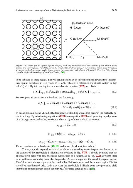
S. Guenneau et al.: Homogenization Techniques for Periodic Structures 11.11 (a) κ 2 N (0,π/2) X (π/2,π/2) X′ (π/4,π/4) Γ (0,0) (b) Brillouin zone κ 1 M′ (0,π/4) M (π/2,0) Figure 11.6: Panel (a) An infinite square array of split ring resonators with the elementary cell shown as the dashed line inner square. Panel (b) shows the irreducible Brillouin zone, in wavenumber space, used for square arrays in perfectly periodic media based around the elementary cell shown of length 2l (l = 1 in (b)). Figure reproduced from Proceedings of the Royal Society [40]. to be the ratio of these scales. The two length scales let us introduce the following two independent spatial variables, ξi = xi/l and Xi = xi/L. The cell’s reference coordinate system is then −1 < ξ < 1. By introducing the new variables in equation (11.6) we obtain, u(X,ξξξ ), ξiξi +Ω2u(X,ξξξ ) + 2ηu(X,ξξξ ), ξiXi +η2u(X,ξξξ ),XiXi = 0. (11.7) We now pose an ansatz for the field and the frequency, u(X,ξξξ ) = u0(X,ξξξ ) + ηu1(X,ξξξ ) + η 2 u2(X,ξξξ ) + ..., Ω 2 = Ω 2 0 + ηΩ 2 1 + η 2 Ω 2 2 + ... (11.8) In this expansion we set Ω0 to be the frequency of standing waves that occur in the perfectly periodic setting. By substituting equations (11.8) into equation (11.7) and grouping equal powers of ε through to second order, we obtain a hierarchy of three ordered equations: u 0,ξiξi + Ω2 0u0 = 0, (11.9) u 1,ξiξi + Ω2 0u1 = −2u 0,ξiXi − Ω2 1u0, (11.10) u 2,ξiξi + Ω2 0u2 = −u0,XiXi − 2u 1,ξiXi − Ω2 1u1 − Ω 2 2u0. (11.11) These equations are solved as in [40, 37] and hence the description is brief. The asymptotic expansions are taken about the standing wave frequencies that occur at the corners of the irreducible Brillouin zone depicted in Fig. 11.6. It should be noted that not all structured cells will have the usual symmetries of a square, as in Fig. 11.6(a) where there is no reflexion symmetry from the diagonals. As a consequence the usual triangular region ΓXM does not always represent the irreducible Brillouin zone and the square region ΓMXN should be used instead. Also paths that cross the irreducible Brillouin zone have proven to yield interesting effects namely along the path MX ′ for large circular holes [39].
Page 1 and 2: GratinGs: theory and numeric applic
Page 3 and 4: Chapter 11: Homogenization Techniqu
Page 5 and 6: Chapter 11 Homogenization Technique
Page 8 and 9: 11.4 Gratings: Theory and Numeric A
Page 16 and 17: 11.12 Gratings: Theory and Numeric

GratinGs: theory and numeric applications - Institut Fresnel

You also want an ePaper? Increase the reach of your titles

Delete template?

Save as template?