Quick start - Gams

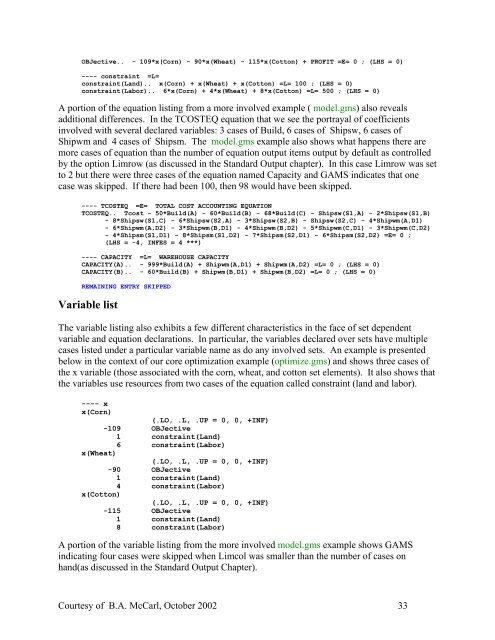
OBJective.. - 109*x(Corn) - 90*x(Wheat) - 115*x(Cotton) + PROFIT =E= 0 ; (LHS = 0)
---- constraint =L=
constraint(Land).. x(Corn) + x(Wheat) + x(Cotton) =L= 100 ; (LHS = 0)
constraint(Labor).. 6*x(Corn) + 4*x(Wheat) + 8*x(Cotton) =L= 500 ; (LHS = 0)
A portion of the equation listing from a more involved example ( model.gms) also reveals
additional differences. In the TCOSTEQ equation that we see the portrayal of coefficients
involved with several declared variables: 3 cases of Build, 6 cases of Shipsw, 6 cases of
Shipwm and 4 cases of Shipsm. The model.gms example also shows what happens there are
more cases of equation than the number of equation output items output by default as controlled
by the option Limrow (as discussed in the Standard Output chapter). In this case Limrow was set
to 2 but there were three cases of the equation named Capacity and GAMS indicates that one
case was skipped. If there had been 100, then 98 would have been skipped.
---- TCOSTEQ =E= TOTAL COST ACCOUNTING EQUATION
TCOSTEQ.. Tcost - 50*Build(A) - 60*Build(B) - 68*Build(C) - Shipsw(S1,A) - 2*Shipsw(S1,B)
- 8*Shipsw(S1,C) - 6*Shipsw(S2,A) - 3*Shipsw(S2,B) - Shipsw(S2,C) - 4*Shipwm(A,D1)
- 6*Shipwm(A,D2) - 3*Shipwm(B,D1) - 4*Shipwm(B,D2) - 5*Shipwm(C,D1) - 3*Shipwm(C,D2)
- 4*Shipsm(S1,D1) - 8*Shipsm(S1,D2) - 7*Shipsm(S2,D1) - 6*Shipsm(S2,D2) =E= 0 ;
(LHS = -4, INFES = 4 ***)
---- CAPACITY =L= WAREHOUSE CAPACITY
CAPACITY(A).. - 999*Build(A) + Shipwm(A,D1) + Shipwm(A,D2) =L= 0 ; (LHS = 0)
CAPACITY(B).. - 60*Build(B) + Shipwm(B,D1) + Shipwm(B,D2) =L= 0 ; (LHS = 0)
REMAINING ENTRY SKIPPED
Variable list
The variable listing also exhibits a few different characteristics in the face of set dependent
variable and equation declarations. In particular, the variables declared over sets have multiple
cases listed under a particular variable name as do any involved sets. An example is presented
below in the context of our core optimization example (optimize.gms) and shows three cases of
the x variable (those associated with the corn, wheat, and cotton set elements). It also shows that
the variables use resources from two cases of the equation called constraint (land and labor).
---- x
x(Corn)
(.LO, .L, .UP = 0, 0, +INF)
-109 OBJective
1 constraint(Land)
6 constraint(Labor)
x(Wheat)
(.LO, .L, .UP = 0, 0, +INF)
-90 OBJective
1 constraint(Land)
4 constraint(Labor)
x(Cotton)
(.LO, .L, .UP = 0, 0, +INF)
-115 OBJective
1 constraint(Land)
8 constraint(Labor)
A portion of the variable listing from the more involved model.gms example shows GAMS
indicating four cases were skipped when Limcol was smaller than the number of cases on
hand(as discussed in the Standard Output Chapter).
Courtesy of B.A. McCarl, October 2002 33