Fernerkundung I (Digitale Bildverarbeitung) - Friedrich-Schiller ...

BSc Geographie
Friedrich-Schiller-Universität Jena
Fernerkundung I
(Digitale Bildverarbeitung)
GEO212
Autor: Dr. S. Hese
Skript zur Übung Fernerkundung-I GEO212, FSU Jena
V 0.71 07112006

Fernerkundung I (Digitale Bildverarbeitung) GEO212
Autor: Dr. S. Hese
Skript zur Übung Fernerkundung I GEO212, FSU Jena
Versioning:
v.0.1 - 8.2004: Initial stuff and structure definition
v.0.2 - 9.2004: Geomatica figures, added section 3
v.0.3 – 10.2004: Minor corrections.
v.0.4 – 11.2004: Automos correction
v.0.5 – 1 .2005: Xpace routines & minor corrections
v.0.6 – 7.2005: Minor changes & V10 Updates
v.0.71 – 11.2006: Minor changes to exercises and some typos corrected
1. Einführung ...................................................................................................... 3
1.1 Inhalt dieses Skriptes ................................................................................... 3
1.2 Theorieinhalte der LV Fernerkundung I GEO212: ......................................... 3
1.3 Digitale Bildverarbeitung – die Grundlagen ...................................................... 5
1.4 Digitale Bildverarbeitung in der Fernerkundung – Komponenten eines
Bildverarbeitungssystems................................................................................... 6
2 Bildverarbeitungssoftware in der Fernerkundung.................................................... 7
2.1 Fernerkundungssoftware............................................................................... 7
2.2 Andere Softwarepakete mit z.T. fernerkundungsrelevantem Funktionsumfang: ... 10
3 Arbeiten mit Geomatica 9 – eine Einführung........................................................ 13
3.1 Die Geomatica Toolbar: .............................................................................. 13
3.2 Mit Xpace arbeiten ..................................................................................... 14
3.3 Arbeiten im Command-Mode (EASI): ............................................................ 15
3.4 EASI/PACE Routinen nach Anwendungsbereichen sortiert ................................ 17
3.5 EASI- Programmierung............................................................................... 29
3.6 GCPWorks ................................................................................................ 31
3.7 ImageWorks – der stabile Image-Viewer aus den 90igern................................ 37
3.8 Geomatica OrthoEngine – creating an ASTER DEM from scratch: ...................... 39
3.9 FOCUS (die integrative Umgebung aller Geomatica Funktionen) ....................... 42
3.10 Die Algorithmenbibliothek – arbeiten mit Geomatica ohne EASI/PACE.............. 46
3.11 Der PCI Modeler....................................................................................... 46
3.12 PCIDSK Datenformat:............................................................................... 47
3.13 Lizenzierung............................................................................................ 50
3.14 Geomatica 10 – ein Ausblick ...................................................................... 52
4. Literatur ....................................................................................................... 53
4.1 National and International Periodicals: .......................................................... 53
4.2 Geomatica spezifische Literaturhinweise: ...................................................... 53
4.3 Lehrbücher: .............................................................................................. 55
4.4 Other References and further reading: .......................................................... 55
4.5 Online Tutorials: ........................................................................................ 58

1. Einführung
1.1 Inhalt dieses Skriptes
Dieses Skript gibt eine Einführung in die Software Geomatica 9.x und 10 und ist Teil der
Dokumentation für ein Vorlesungsskript zum Modul Fernerkundung I des BSC Geographie
an der Friedrich-Schiller-Universität Jena. Teile dieser Dokumentation wurden der
EASI/PACE Hilfe von Geomatica und online Material von http://www.pci.on.ca
entnommen bzw. von CGI-Systems zur Verfügung gestellt oder stammen aus
Aufzeichnungen von S. Hese.
Die vorläufige Planung sieht z.Zt. folgende Übungen mit Geomatica Software vor:
• Ü1: Datenimport und PCIDSK Database Management - Layerstacking /
Einführung in das XPACE BV-System
• Ü2: Database handling (ASL, CDL, MCD, LOCK, UNLOCK), PCIDSK File
Management mit PCIMOD
• Ü3: Georeferenzierung / geometrische Korrektur - Arbeiten mit GCPWorks
• Ü4: NDVI, Ratios und PCA (PCIMOD, MODEL, THR, MAP, ASL, CDL, PCA)
• Ü5: Filterungen im Ortsbereich (PCIMOD, EASI/PACE Database Filtering)
• Ü6: Filterungen im Frequenzbereich (PCIMOD, FTF, FFREQ, FTI)
• Ü7: IHS Data Fusion (PCIMOD, FUSE, IHS, RGB)
• Ü8: Klassifikation I – supervised classification (MLC, CSG, CSR, CHNSEL, SIGSEP,
PCIMOD, SIEVE)
• Ü9: Klassifikation II – unsupervised classification (Clustering), (PCIMOD,
ISOCLUS, KCLUS)
• Ü10: Texturanalyse (PCIMOD, TEX)
• Ü11: Genauigkeitsanalysen (User – Producer Accuracy, MLR, MAP)
1.2 Theorieinhalte der LV Fernerkundung I GEO212:
1. Einführungsveranstaltung: Vorbesprechung, Allgemeines, Informationen zu den
Übungen und Tutorien, Lehrveranstaltungsinhalte, Literatur, Übungslisten,
Gruppenaufteilung.
2. Termin: Einführung in die Software Geomatica (EASI/PACE, XPACE, Modeler,
Focus, GCPWORKS, EASI Programmierung), Einführung in das menschliche Sehen
und Bildverstehen, Reizverarbeitung, Aufbau des Auges, Stäbchen, Zapfen,
Farbsehen, menschliche Signalverarbeitung, Stereobildverarbeitung, Technologie
digitaler Sensoren, CCD Sensor Architektur, Zeilensensor ver. Framesensor, Farbe
bei der digitalen Datenaufnahme, CCD und CMOS Sensor und Aufnahmesysteme,
Sensor Architekturen, Fillfaktor,
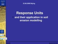
3. Termin: Grundlagen der digtialen Bild- und Signalverarbeitung, Grundlagen der
Fernerkundung (compressed), Sensorik zwischen räumlicher und spektraler
Auflösung, Detektorkonfigurationen, das Pixel, Datenspeicherung, Datentypen,
Datenformate, Dateneinheiten, Bit, Byte, Megabyte, Datensatzgrößenberechnung,
BSQ, BIL, BIP, Anwendungen, Vor- und Nachteile, Auflösungsarten (räumlich,
spektral, radiometrisch, temporal), Software in der digitalen Bildverarbeitung –
ein Überblick, Byte Order, Bildpyramiden, Einführung in das Histogramm,
Prozesse in der industriellen BV und in der Fernerkundung, Fernerkundungs-
Bilddateiformate, das PCIDSK Dateiformat, Arbeiten mit Segmenten in Geomatica.
4. Termin: Datenvorverarbeitung: geometrische Korrektur, parametrische Verfahren,
Interpolationsverfahren, geometrische Verzerrungen bei Satellitendaten und
Flugzeugdaten, Entzerrung, Resamplingverfahren (NN BIL, CC), Polynome erster
und nter Ordnung, der RMS Error, systematische Korrektur von

Zeilenscannerdaten, Detaileinführung GCPWorks, Übung mit GCPWorks in
Geomatica (Image to Image Correction).
5. Termin: Histogramm Transferfunktionen, das Histogramm, Lookup Tables,
Histogramm Equalisation, Linear Stretch, Äquidensitenstreckung, Histogramm
Thresholding, Histogramm Matching, Brightness Inversion, radiometrische
Kalibrierung, Atmosphärenkorrektur Überblick über verschiedene Ansätze (Modell
basiert, Dark-Pixel Subtraction, Empirical Line), Vorteile der AK,
Strahlungskomponenten, Units of electromagnetic radiation: "Radiant Flux
Density per Unit Area per Solid Angle, mW cm-2 sr-1 um-1 (= spectral
radiance)), Gain-Settings, Reflectance vers. Radiance. ATCOR2 in Geomatica,
ATCOR2 und ATCOR3, topographische Korrektur (Kanalratios, mit lokalem
Beleuchtungswinkel, Berechng. des Einfallswinkels, Lambertsche Methode, Civco
Modifikation, Non-Lambertsche Methode mit Minneart Konstante,
6. Termin: Spektrale Transformationen, spektrale Eigenschaften von Vegetation,
Aufbau eines Blattes, Vegetationsindizes, Red Edge, NDVI (Normalized Difference
Vegetation Indice) und andere Ratios, HKT (Transformation) - PCT (Principal
Component Transformation, Theorie und Beispiele für praktische Anwendungen,
Tasseled Cap Transformation im Vergleich zur PCT - Vorteile und Nachteile,
Kanalratios und PCT in Geomatica und EASI/PACE, Übung zur PCA in XPACE,
7. Termin: Räumliche Transformationen, Filterungen im Ortsbereich, Image Domain
Filterverfahren, Randpixelproblematik, Highpass, Lowpass, Highboost etc.,
statistische Filter (Mean, Median, Gaussian, MinMax), morphologische Filter,
Kantendetektoren, Zero-Sum Filter (Laplace, Sobel, Prewitt, subtraktive
Glättung), adaptive Filterverfahren (Frost, Lee), Filterungen in Geomatica,
Übungen zu Highpass, Lowpass und ZeroSum-Filterungen in EASI/PACE und
Imageworks,
8. Termin: Filterungen im Frequenzraum, Fourier-Transformation, Step-Funktion, 1-
D-Step-Funktion und Umsetzung durch Amplitude und Frequenz, 2-D DFT, die
Fouriersynthese, Phase und Magnitude, Powerspektrum, Reduzierung von
Bildrauschanteilen, SNR (Signal to Noise), FFT in Geomatica, Übung zur
Noisereduzierung mittels Medianfilter und Fourier Transformation unter
Verwendung von EASI/PACE Programmmodulen,
9. Termin: Datenfusion, Auflösungsproblematik: high res. spectral vers. spatial
resolution, Datenfusionsprozesstypen, Ziele der Datenfusion, IHS, Hexcone
Farbmodel, Farbraum-Projektion, Intensity, Hue, Saturation, PCA/PCS Fusion
(Principal Component Substitution - PCS), COS-Verfahren, Pansharpening,
Arithmetische Kombinationen - Fusion, Theorie die Farbraumtransformationen,
HIS-RGB in Geomatica, SVR Fusion, Übung zur Datenfusion in EASI/PACE.
10. Termin: Parametrische Klassifikatoren: Gliederung der Klassifikationsverfahren
(unüberwachte -überwachte Verfahren; parametrische - nicht-parametrische
Verfahren), unüberwachtes Clustering, K-Means, ISODATA, Min Distance to Mean,
Parallelepiped Classifier, MLC (Maximum Likelihood Klassifikation),
Verfahrensgliederung bei der überwachten Klassifikation (Definition von
Trainingsgebieten, Definition von Evaluierungs(Test)gebieten,
Genauigkeitsanalyse), kombinierte Verfahren, Postklassifikations Smoothing,
ISODATA Clustering in Geomatica, Übung zur unüberwachten Klassifikation in
Geomatica (EASI/PACE),
11. Termin: Nicht parametrische Verfahren, Gliederung der Klassifikationsverfahren
(unüberwachte -überwachte Verfahren; parametrische - nicht-parametrische
Verfahren), Level Slicing, (Box-Classifier), ANN (Artifical Neural Networks) -
Einführung in Theorie, Anwendungen und Programme in EASI/PACE,
Prozessablauf in XPACE, Problembereiche bei der Anwendung, Struktur der
Klassifikation mit ANNs (Konstruktion, Trainingsphase, Klassifikationsphase,
Hierarchical Classification, NN Klassifikator, Distance-Weighted k-NN, Narenda
Goldberg non-iteratives und nicht-parametrisches Histogramm Clustering,

Descision Tree Klassifikatoren, DTC vers. ANN, ANN Module in Geomatica
(Beschreibung der Advanced ANN Module in EASI/PACE), Übung zur überwachten
Klassifikation,
12. Termin: Textur, Definitionen, statistische Parameter 1er Ordng (Varianz,
Mittelwert), statistische Parameter 2ter Ordng. (SGLD), Spatial Grey Level
Dependence Matrices, Concurrence Matrix, Co-occurence Matrix, SGD-Matrix-
Klassen: Contrast, Dissimilarity, Homogenität, Angular Second Moment (Energy,
Entropy), GLCM Mean, Variance, Stdev, Correlation), statistische Parameter 3ter
und nter Ordng. (Variogrammanalysen und -texturklassifikation), Textur zur
Datensegmentierung, Link zu Segmentierungsmethoden, Mustererkennung,
Textur in Geomatica (Modulüberblick und -anwendung von TEX ), Übung zur
Texturklassifikation in EASI/PACE,
13. Termin Genauigkeitsanalysen von Klassifikationsergebnissen
(Evaluierungsgebiete, Trainingsgebiete, User- und Producer Genauigkeit, Error of
Omission, Error of Comission, MLR (Maximum Likelihood Report) in Geomatica,
Übung zur Klassifikationsgenauigkeit, Literaturhinweise zum Thema,
14. Termin: Hyperspektrale Datenauswertung, Eigenschaften, Sensoren
(Kurzüberblick), Datenredundanz, spectral Unmixing, Endmembers, Spectral
Angle Mapper, MNF (Minimum Noise Fraction), Spectral Feature Fitting, Binary
Encoding, Hyperspektrale Datenverarbeitung in ENVI und SAM in Geomatica,
Ausblick auf die Objekt orientierte Klassifikation und Schnittmengen mit GIS
(Landscape Metrics, Fragstat, r.le in GRASS), ULE (Lehrevaluierung),
15. ggf. 15. Termin: Wiederholung aller Termininhalte in komprimierter Form,
Fragestunde zur Klausur, Ergebnis-Diskussion der ULE Analyse
1.3 Digitale Bildverarbeitung – die Grundlagen
Einheiten der Speicherkapazität:
1 Bit = -> 0 oder -> 1 - ( Ja ) oder ( Nein )
1 Byte = 8 Bit = 1 Zeichen (=> 256 mögliche Ausprägungen)
1 KiloByte = 1024 Bytes -> 1024 = 2(hoch 10)
1 MB = 1 Megabyte = 1024 * 1024 Byte (1.048.576 Byte).
Megabyte:
Die Berechnung von einem Megabyte führt immer wieder zur Verwirrung,
daher sei hier auf den Faktor hingewiesen, mit dem gerechnet werden muss:
1024 Byte = 1 KiloByte,
1024 KiloByte = 1 Megabyte.
1024 Megabyte = 1 Gigabyte
Um also von z.B. 123.456.789 Bytes auf Megabyte umzurechnen,
rechnet man: (123.456.789/1024)/1024=117,73 MB, oder
123.456.789/1048576=117,73 MB
Dieser Faktor wird in allen Berechnungen, die in MegaByte ausgedrückt werden,
verwendet. Unglücklicherweise halten sich z.B. einige Hardwarehersteller nicht an diese
Konvention. Dies führt beim Kauf von Festplatten immer wieder zu Verwirrungen.

KB=
1024
Byte
Kilobyte 2^10 = 1.024 Bytes ca. 1
Tausend
(ca.
10^3)
MB=
1024
KB
Megabyte 2^20 = 1.048.576 Bytes ca. 1 Million
(ca.
10^6)
GB=
1024
MB
Gigabyte 2^30 = 1.073.741.824 Bytes ca. 1
Milliarde
(ca.
10^9)
TB=
1024
GB
Terabyte 2^40 = 1.099.511.627.776 Bytes ca. 1 Billion
(ca.
10^12)
PB= 1024 TB Petabyte 2^50 = 1.125.899.906.842.624 Bytes ca. 1
Billiarde
(ca.
10^15)
EB= 1024 PB Exabyte 2^60 =
1.152.921.504.606.846.976
Bytes
ca. 1 Trillion
(ca.
10^18)
ZB= 1024 EB Zetabyte 2^70 =
1.180.591.620.717.411.303.4
24 Bytes
ca. 1
Trilliarde
(ca.
10^21)
YB=
1024
ZB
Jotabyte 2^80 =
1.208.925.819.614.629.174.7
06.176 Bytes
(ca.
10^24)
Im Gegensatz zur Beschreibung von Datenmengen, spricht man bei der Beschreibung
der radiometrischen Datenauflösung nur von Bit und nicht von Byte (8Bit) Einheiten.
Es gilt also:
1 Bit (on or off) 2 1 (2 mögliche Ausprägungen)
8 Bit 2 8 values, equals 1 Byte (256 Werte - 0-255)
10 Bit 2 10 values, 1024 Werte
12 Bit 2 12 values, 4096 Werte
16 Bit 2 16 (2 Byte), 65536 Werte
32 Bit 2 32 (4 Byte), 4.294.967.296
64 Bit 2 64 (8 Byte), 18.446.744.073.709.551.616
128 Bit 2 128 (16 Byte)
Type Descriptions:
integer 4 byte signed integer number
float 4 byte single precision floating point number
double 8 byte double precision floating point number
char single character (1 byte)
byte single unsigned byte (8 Bit)
1.4 Digitale Bildverarbeitung in der Fernerkundung – Komponenten eines
Bildverarbeitungssystems
Die Methoden der digitalen Bildverarbeitung werden in der Fernerkundung aufgeteilt in
unterschiedliche in einer spezifischen Reihenfolge abzuarbeitende Prozessierungs- oder
Verarbeitungsschritte:
1. Image Preprocessing:
a. Noise Removal
b. Geometric Correction / Geocoding / Georeferencing

c. Radiometric Correction
d. Atmospheric Correction
e. Topographic Normalisation
2. Image Enhancement:
a. Contrast Manipulation
b. Spatial Feature Manipulation
c. Multi Image Manipulation
d. Data Fusion
e. Multispectral Transformation
f. Feature Reduction
3. Image Classification and/or Biophysical Modelling
a. Supervised classification
b. Unsupervised classification
c. Biophysical parameter retrieval (Biomass, FPAR, LAI, forest stand density
etc.)
Bilddaten in der Fernerkundung haben spezifische Merkmale. Im Einzelnen lassen sich
folgende Merkmalsbereiche voneinander trennen:
• Radiometrische – spektrale Merkmale
• Geometrische – texturelle Merkmale
• Temporale Merkmale
• Kontextmerkmale
2 Bildverarbeitungssoftware in der Fernerkundung
2.1 Fernerkundungssoftware
ENVI/IDL:
Schwerpunkt der Analysefunktionen in ENVI ist der hyperspektrale Bereich. Ein großer
Vorteil von ENVI ist die nahtlose Integration von IDL Routinen in ENVI. IDL gilt im
Bereich der Fernerkundung als eine der stärksten Programmiersprachen. Im Vergleich zu
anderen Umgebungen fällt bei ENVI die enorme Menge an Fenstern auf, mit denen
Eingaben und Darstellungen umgesetzt werden. Oft werden wichtige Funktionen tief in
Menüstrukturen versteckt. Intensives Arbeiten führt schnell zu sehr unübersichtlichen
Desktops und erschwert erheblich das systematische Arbeiten. Der Viewer von ENVI ist
recht schnell und solange man nicht mit mehreren Datensätzen arbeitet ist das Konzept
sehr ergonomisch bedienbar. Problematisch wird es, wenn mehrere Datensätze angezeigt
werden sollen (Übersichtlichkeit). Die hyperspektrale Funktionalität ist wohl am Markt
führend. Nutzung und Entwicklung eigener IDL Routinen ist jedoch nötig, um das
eigentliche Potential der Softwareumgebung auszunutzen. Mit der Version 4.0 ist einiges
an Funktionalität hinzugekommen (Decision Tree Classifier, Neural Net Classifier). Die
Unterstützung von Fremdformaten ist erheblich besser geworden mit den neueren
Versionen ab 3.5. Das ENVI Bilddatenformat ist recht einfach über eine ASCII-Header-
Datei ansprechbar und es existiert ein eigenes Vektorformat. Die Stabilität ist
befriedigend. Z.T. existieren Erweiterungen, die jedoch kostenpflichtig sind (z.B. ASTER
DTM). Demoversion ist vollständig herunterladbar, arbeitet jedoch nur 7 Minuten lang.
Der Creaso-Support ist vorbildlich (www.creaso.com). Es existiert eine Studentenversion
zu erheblich reduziertem Preis.

Fazit: ENVI ist die Entwicklungsumgebung der Wahl für alle Arbeiten im Bereich der
hyperspektralen Datenverarbeitung und -analyse. Aufgrund der Nähe zu IDL auch in
vielen anderen Bereichen der Fernerkundung sehr oft eingesetztes Softwarepaket.
Schnelle Einarbeitung möglich. Funktionsumfang in Version 4.0 hat gleichgezogen mit
anderen RS-Software-Paketen. Insbesondere die Verfügbarkeit von IDL ist i.d.R. ein
entscheidendes Kaufargument.
ERDAS Imagine:
Zur Leica Geosystems Gruppe gehörendes Softwarepaket mit viel Tradition im
deutschsprachigen Raum. Kein spezifischer Schwerpunkt, jedoch gute Funktionalität im
Bereich Photogrammetrie und allgemeine Fernerkundung. Die Nutzung von Modeller und
EML Programmierungen zur Erweiterung der Funktionalität ist in den meisten Fällen
notwendig. Der grafische Modeller ist sehr gut gelungen und sehr flexibel einsetzbar.
Einige spezielle Tools (Knowledge Engineer, Knowledge Classifier) und die ATCOR
Einbindung (AddOn) sind herauszustellen. Schwache Leistung im Bereich
Vectordatenverarbeitung (Vector Modul ist von ArcINfo eingekauft und bringt nur wenig
Funktionalität aus ArcInfo mit und ist unverständlich teuer), dafür aber sehr ausgereiftes
Tool für 3D Visualisierung (VirtualGIS). Nicht vollständige Importfunktion für die
gängigen Datenformate (Geomatica PCIDSK?). Sehr schneller und stabiler Viewer.
Warum gibt es so einen Viewer nicht auch in anderen Software-Lösungen? Die
Dokumentation ist jedoch definitiv nicht ausreichend, insbesondere die Online- bzw.
Kontexthilfe taugt i.d.R. gar nicht bzw. hilft einem nicht weiter. Webseite unter:
(http://www.gis.leica-geosystems.com/Products/Imagine/). Große Usergemeinde in
Deutschland, aber auch in den USA. Regelmäßige Nutzertreffen in Deutschland durch
Geosystems organisiert. Email-Forum mit reger Teilnahme. Support über Geosystems in
München. Stabilität zufrieden stellend und eindeutig besser als bei der Geomatica 9.x
Reihe.
Fazit: Guter Einstieg in die Fernerkundung, jedoch nicht das systematische Arbeiten
unterstützend. Gewohntes Bedienkonzept vieler Menüs, klasse Pfadnavigationsoptionen,
die zu erheblich beschleunigtem Arbeiten führen. Vorbildlicher Datenviewer und sehr
guter grafischer Modeller im Baukasten System.
ERMapper:
Aus Australien stammende Software mit Stärken im Bereich der Visualisierung. Im
zentraleuropäischen Bereich nicht sehr stark vertreten, jedoch mit großer
Funktionsvielfalt. Demoversion downloadbar. Bekannt wurde in den letzten Jahren das
Dateiformat ECW, ein auf Waveletmethoden basierendes Dateiformat mit hohen
verlustfreien Kompressionsraten. Sehr gute Visualisierungstools für GIS Daten und 3D
Information.
eCognition:
Objektorientierte Bildverarbeitung (Segmentierung & Klassifikation von Bildsegmenten
ohne klassische Datenverarbeitungsfunktionen wie z.B. Atmosphärenkorrektur oder
geometrische Korrektur. eCognition wird von der Firma Definiens aus München
vertrieben (http://www.definiens-imaging.com/ecognition/pro/index.htm) und empfiehlt
sich in erster Linie für geometrisch sehr hoch auflösende Datensätze im Bereich 1-15 m
und höher auflösend. Gute Dokumentation, hohe Anforderungen an die Hardware,
komplexe Einarbeitungsphase möglichst mit erheblichen Vorkenntnissen aus der BV
notwendig. Jährliche Nutzertreffen in München oder anderswo, online Mailforum. Netter
Support aus München, jedoch nicht immer verfügbar (i.d.R. wird man auf das Online-
Interface vertröstet). Vollständige Demoversion downloadbar (Begrenzung nur durch die
Bildgröße). Stabilität der Software sehr gut bei kleineren Datensätzen – eher sehr

schlecht bei sehr großen Datensätzen. LDH Version verfügbar, die die 32Bit
Adressraumbegrenzung von Windows XP 32 überwindet.
Fazit: Software für spezielle Fragestellungen. Zur vollständigen Nutzung aller Funktionen
sind erhebliche Erfahrungen im Bereich der Bildverarbeitung und möglichst auch im GIS
Bereich Voraussetzung.
Geomatica 9.x (Ex PCI):
Produkt der kanadischen Softwarefirma PCI-Geomatics mit langer Tradition im
Erdfernerkundungsbereich. Unterschiedliche Nutzerinterface machen es dem Einsteiger
schwer, den richtigen Weg in die Funktionalität der Software zu finden. Wer jedoch eine
flache und anstrengende Lernkurve zu Beginn überstanden hat, dem stehen viele
Funktionen zur Verfügung, die sich einfach über Routinen einbinden lassen und für viele
Anwendungen anpassbar sind. EASI Programmierumgebung kann zur Entwicklung von
Batch Prozessierungsroutinen genutzt werden. Durch die Nähe der EASI/PACE und
XPACE Routinen zur EASI-Programmierung ist der Einstieg in die Programmierung von
Routinen recht einfach. Das Nutzerinterface zwingt den Anwender Verfahren und
Methoden vollständig zu verstehen. Die Onlinehilfe ist absolut notwendig für Einsteiger.
Der Funktionsumfang vieler Routinen ist erheblich und sehr gut konfigurierbar. Sehr gute
Datenimportfunktionen für praktisch fast alle Fremdformate (inklusive Erdas Imagine).
Sehr guter OrthoEngine mit automatischer Unterstützung vieler Sensor-Daten-
Geometrien. Die Onlinehilfe ist vorbildlich gelöst und enthält auch weitergehende
Literaturhinweise und ist durch die automatische Mitführung der Hilfe unter Xpace sehr
hilfreich um die Lernkurve zu verbessern. Online-Hilfe von Focus leider nicht in der
gleichen Tradition aufgebaut. Der grafische Modeller ist im Konzept sehr gut, leider im
Funktionsumfang noch eingeschränkt (in Version 10 ausgebaut worden).
Leider existieren in der Version 9.x immer noch Probleme mit der Stabilität bei
Verwendung des Focus Interface bzw. mit der grafischen Darstellungsqualität unter
UNIX. ATCOR Einbindung nicht so gut gelungen wie in ERDAS (wie kann man effektiv c0
und c1 Koeffizienten erzeugen?). Topografische Normalisierung mittels DTM fehlt als Tool
(aber in ATCOR3 verfügbar – kostenpflichtiges „Advanced Modul“). Das Focus Viewer
Interface ist sehr langsam und hat auch nach Updates i.d.R. noch erhebliche Bugs. Der
Updatezyklus ist recht schnell. I.d.R. erscheinen vierteljährliche Bugbereinigungen.
Demoversion von Geomatica ist bestellbar. Ein abgespeckter Viewer ist frei verfügbar.
Große Usergemeinde insbesondere im englischen Sprachraum (Kanada, GB, USA).
Nutzertreffen in Deutschland eher selten (CGI-Systems). Fortbildungen i.d.R. in Canada
oder GB. Waches Email-Forum mit Austausch von EASI Skripten ist herauszustellen.
Support in Deutschland über CGI Systems in München. Website unter: (www.pci.on.ca).
Fazit: Softwarepaket für Anwender mit Nähe zur Programmierung, da die volle
Funktionalität erst durch EASI-Routinen nutzbar ist. Komplexe Einarbeitungsphase
notwendig, da das Nutzungskonzept viel Vorwissen voraussetzt. PCI unterstützt jedoch
entscheidend das methodische und strukturierte Arbeiten mit Fernerkundungsdaten
durch den sehr modularen Aufbau. Schade, das der Rest des Konzeptes nach Version 6.0
so unglaublich instabil läuft. Dies soll in der Version 10 besser geworden sein.
VICAR:
Das VICAR Bildverarbeitungssystem wurde am JPL entwickelt und wird genutzt, um
Daten der Planetenmissionen z.B. zum Mars auszuwerten. VICAR ist komplett
Kommandozeilen orientiert und gut scriptierbar.
“VICAR, which stands for Video Image Communication And Retrieval, is a general
purpose image processing software system that has been developed since 1966 to
digitally process multi-dimensional imaging data. VICAR was developed primarily to
process images from the Jet Propulsion Laboratory's unmanned planetary spacecraft. It

is now used for a variety of other applications including biomedical image processing,
cartography, earth resources, astronomy, and geological exploration. It is not only used
by JPL but by several universities, NASA sites and other science/research institutions in
the United States and Europe.”. Kein Support, nach Kenntnisstand kein Mailforum.
http://www-mipl.jpl.nasa.gov/external/vicar.html
KHOROS:
„Khoros Pro 2001 (http://www.khoral.com/) ist eine Softwareentwicklungsumgebung,
mit der aus einem Repertoire an vorhandenen Softwarebausteinen eigene Applikationen
entwickelt werden können. Die Anwendungsschwerpunkte liegen dabei in den Bereichen
Bildverarbeitung, Signalverarbeitung und Visualisierung.
Khoros war ursprünglich eine Entwicklung der University of New Mexico (1990) und
wurde lange Zeit im Quelltext zum freien Download zur Verfügung gestellt. Dadurch
erreichten die ursprüngliche Version 1 sowie die Nachfolgeversion Khoros 2 auch in
Deutschland einige Verbreitung bei Hochschulinstituten und Forschungseinrichtungen.
Seit einigen Jahren wird Khoros nun von einer eigens gegründeten Firma als
kommerzielles Produkt weiterentwickelt und vertrieben (Khoral Research Inc.).
Den Vertretern von Khoral Research ist dabei wohl bekannt, dass ein nicht
unwesentlicher Teil des Khoros-Systems aus Entwicklungen einer aktiven
Nutzergemeinde entstanden ist, die im Laufe von Jahren viele Bausteine zu dem Paket
beigetragen hat. Außerdem gründete die Attraktivität der ersten Khoros-Versionen nicht
zuletzt auf der Verfügbarkeit der Programmquellen. Unter diesem Aspekt bietet Khoral
Research Inc. auch weiterhin eine "Studentenversion" im Quelltext an, die sich
Studenten nach einer Registrierung herunterladen können, die aber nicht weiterverteilt
werden darf. Diese besteht aus dem Quelltext einer Beta-Version von Khoros Pro, die
aktuelle Weiterentwicklungen in einer frühen Testphase beinhaltet“ (http://www.lrzmuenchen.de/services/software/grafik/khoros/).
Inzwischen ist Khoros in den Besitz von AccuSoft übergegangen und nicht mehr frei
verfügbar. Das System heißt nun wohl VisiQuest (http://www.accusoft.com/) und ist voll
kommerziell.
Fazit: Sehr schade, dass Khoros nicht mehr „freie“ Software ist!
2.2 Andere Softwarepakete mit z.T. fernerkundungsrelevantem
Funktionsumfang:
GRASS:
GRASS ist ein Open Source GIS (http://grass.baylor.edu/), welches frei verfügbar ist.
Vollversion herunterladbar. Auch für unterschiedliche UNIX Varianten kompilierbar.
Windows Portierung unter Verwendung von Cygwin.
“GRASS GIS (Geographic Resources Analysis Support System) is an open source, Free
Software Geographical Information System (GIS) with raster, topological vector, image
processing, and graphics production functionality that operates on various platforms
through a graphical user interface and shell in X-Window. It is released under GNU
General Public License (GPL).”
Alle Module sind in den GRASS-Manpages beschrieben. Funktionalitäten im Bereich
Bildverarbeitung (Image Processing): Auflösungsverbesserung, Bildentzerrung (affin,
polynomisch) auf Raster- oder Vektorgrundlagen, Farbkomposite, Fouriertransformation,
Hauptkomponentenanalyse (PCA), Histogrammstreckung und -stauchung, Image Fusion,
kanonische Komponentenanalyse (CCA), Kantenerkennung, Klassifikationen: (a)
radiometrisch: unüberwacht, teilüberwacht und überwacht (Affinity, Maximum
Likelihood), (b) geometrisch/radiometrisch: unüberwacht (SMAP), Kontrastverbesserung,
Koordinatentransformation, IHS/RGB-Transformation, Orthofoto-Herstellung,
Radiometrische Korrektur (Filterung), Resampling (bilinear, kubisch, IDW, Splines),

Shape Detection, Zero Crossing. Visualisierungsmöglichkeiten: Animationen, 3D-
Oberflächen, Bildschirm-Kartenausgabe, Farbzuweisung, Histogramm.
Nutzergemeinde praktisch nur UNIs, rege Aktivitäten in den Mailforen, jedoch viele
wiederkehrenden Probleme mit Portierungshintergrund. Kaum Schulungen, online tutorial
ist sehr gut. Handbücher verfügbar. Support gibt’s nicht (Open Source), Nutzertreffen
nach Bedarf und Laune). Große Stärke ist die Integration eigener Skriptroutinen unter
UNIX (UNIX Shell und Utilities sind vollständig nutzbar). TclTk Interface nach eigenen
Vorstellungen ausbaubar.
Fazit: Eine Umgebung für die Entwicklung von GIS-Routinen, Schwerpunkt im Raster-GIS
Sektor.
ArcGIS:
Das GIS Software Paket schlechthin, mit nicht endenden Funktionen, Schnittstellen und
Ausbaustufen vom Marktführer im GIS-Sektor ESRI (www.esri.com). Rasterfunktionalität
kommt mit den ArcGIS Extensions: Spatial Analyst (find suitable locations, find the best
path between locations, perform integrated raster/vector analysis., Perform distance and
cost-of-travel analyses, perform statistical analysis based on the local environment,
small neighbourhoods, or predetermined zones, generate new data using simple image
processing tools, interpolate data values for a study area based on samples, clean up a
variety of data for further analysis or display; 3D Analyst; Geostatistical Analyst;
ArcScan (Perform automatic or interactive raster-to-vector data conversion, create
shapefile or geodatabase line and polygon features directly from raster images, use
raster snapping capabilities to make interactive vectorization more accurate and efficient,
prepare images for vectorization with simple raster editing).
Schwerpunkt der Rasterfunktionen in ArcGIS liegt auf GIS Analysefunktionen,
Datenaustausch, Interpolation, nicht auf der klassischen Bildverarbeitung und dem Data
Preprocessing.
Halcon:
(http://www.mvtec.com/halcon/) Software mit Schwerpunkt im Bereich industrielle
Bildverarbeitung und Feature Detection, Pattern Matching.
„HALCON is well known as a comprehensive machine vision software that is used
worldwide. It leads to cost savings and improved time to market: HALCON's flexible
architecture facilitates rapid development of machine vision and image analysis
applications. HALCON provides an extensive library of more than 1100 operators with
outstanding performance for blob analysis, morphology, pattern matching, metrology, 3D
calibration, and binocular stereo vision, to name just a few.”
IPW:
IPW (Image Processing Workbench) ist ein Bildverarbeitungssystem, das unter UNIX auf
Skript orientierter Arbeitsweise beruht. Diverse Einzelroutinen (um 80) können zu
komplexeren Skripten kombiniert werden. Dokumentation vorhanden (www), online
Version frei verfügbar. Support n/a und Mailforum nicht vorhanden. Stabilität wohl gut –
wenig im deutschen Sprachraum genutzt. Schlechte Schnittstelle zu anderen
Datenformaten (GRASS und UNIX Bildformate), aber sehr gute Unterstützung bei der
Strahlungsmodellierung. Basiert in hohem Maße auf der UNIX Shell. Mit UNIX
Shellprogrammen können schnell und effektiv eigene Routinen zusammengestellt
werden.
“The Image Processing Workbench is a Unix-based image processing software system.
The system was written by Jim Frew, with contributions from Jeff Dozier, J. Ceretha
McKenzie, and others at the University of California, Santa Barbara. The software is

portable among Unix systems and is freely distributable. The name Image Processing
Workbench reflects the influence the Unix system had on the design of IPW, since an
early version of Unix was called the `Programmer's Workbench'.
Individual Unix and IPW programs are "tools" which may be used together to perform
more complicated operations. IPW is a set of programs, written in C, that form an
extension of Unix. Therefore, IPW programs can be used in combination with Unix
programs, and IPW has no need to duplicate basic Unix functions such as file
management and command interpretation.
Unix programs are executed by typing the name of the program as a command to the
shell. Parameters are specified on the command line, rather than in response to user
prompts. The command syntax for IPW is patterned after the proposed standard for Unix
system commands. In Unix and IPW most input and output are on preconnected
channels, the standard input (stdin) and the standard output (stdout). "Pipes" connect
the standard output of one command to the standard input of the next. The use of pipes
avoids intermediate files and speeds the execution time since the second program in the
pipeline may start running as soon as output from the first program begins.”
(http://www.icess.ucsb.edu/~ipw2/crrel.man/1/ipw.html)
Idrisi:
(http://www.clarklabs.org/IdrisiSoftware.asp?cat=2):
Raster Vector-GIS Funktionalität, z.T mit eingeschränkter Kompatibilität mit
kommerziellen Datenformaten.
ILWIS:
ILWIS integrates image, vector and thematic data in one package on the desktop. ILWIS
delivers import/export, digitizing, editing, analysis and display of data as well as
production of quality maps and geostatistical tools. As from 1st January 2004 ILWIS
software will be distributed solely by ITC as shareware to all users irrespective of their
relation with ITC. Documentation is online available.
MATLAB:
MATLAB ® und die Image Processing Toolbox unterstützen eine Vielzahl fortschrittlicher
Bildverarbeitungsfunktionen. Es können Bildmerkmale extrahieren und analysieren,
Merkmalmessungen berechnen und Filteralgorithmen angewendet werden.
MATLAB bietet eine umfangreiche Entwicklungsumgebung, mit Schwerpunkten im
Bereich Algorithmusentwicklung und Anwendungseinsatz, Visualisierung, Bildanalyse und
Verbesserung und Datenim- und export.
Durch Zugriff auf andere Extensions von MATLAB (Neural Network Toolbox u.a.) ist eine
Ausweitung in andere Methodenbereiche möglich. Durch die stark auf Programmierung
basierende Struktur von MATLAB ist diese Software stark vertreten in den technischen
Wissenschaften (Engineering). Ausgedehnte Dokumentation, Software portiert auf
unterschiedliche Betriebssysteme, an vielen Universitäten verfügbar i.d.R. über beliebig
viele Campuslizenzen. Ernsthafte Alternative zu IDL für die Algorithmenentwicklung,
jedoch ohne fertige Standard –Fernerkundungsroutinen. http://www.mathworks.de
/applications/imageprocessing/.
Andere interessante Softwarepakete im GIS/RS Sektor: CARIS, MAPINFO, MANIFOLD,
SMALLWORLD, GMT, VARIOWIN, GSTAT, GSLIB.

3 Arbeiten mit Geomatica 9 – eine Einführung
Dieser Abschnitt wurde z.T. aus den Handbüchern von EASI/PACE und Schulungsmaterial
von CGI Systems 2004 übernommen bzw. stammt aus persönlichen Aufzeichnungen der
Jahre 1995 – 2003 des Autors.
Die Schnellkonfiguration:
* Focus Autostart ausschalten: \etc\geomatica.prf „Autolaunch“ für Focus löschen (1. Zeile)
* Arbeitsverzeichnis von Geomatica Geomatica-Icon/rechte Maus/Ausführen in d:\ Name_Directory
* Focus Nutzereinstellungen Focus/Tools/Options
3.1 Die Geomatica Toolbar:
Über die Geomatica Toolbar werden die Geomatica-Module aufgerufen:
Abb. 1: Geomatica 9.1 Toolbar
Von links nach rechts:
Focus: Datenvisualisierung, Datenerfassung, Datenbankmanagement, Im/Export,
Subset, Reproject, Klassifizieren, Programme ausführen in der Algorithmenbibliothek,
Modeler: Visuelles bzw. graphisches Modellierinterface (vegleichbar mit dem ERDAS
Modeller) auch mit Batch-Processing Fähigkeiten, EASI: Command-Mode Interface und
Programmierumgebung für EASI Routinen (sehr wichtig für Batchprocessing),
OrthoEngine: geometrische Entzerrung, manuelles und automatisches Mosaikieren,
Orthobild und DGM-Generierung, FLY: 3D fly-through, Chip Manager: Erstellung von
Passpunkt-Datenbanken, License Manager: Lizenzierung; ImageWorks: der alte Viewer
von PCI bis zur Version 6. Wird durch Focus ersetzt und fällt wohl in der Zukunft weg;
Xpace: EASI/PACE Routinen mit graphischem Interface – gleiche Softwareumgebung wie
in EASI; GCPWORKS: Tool zur geometrische Korrektur, zur Mosaikierung und
Georeferenzierung.
Die PCI Geomatics Generic-Database-Technologie erlaubt den Zugriff auf über 100
Raster- und Vektorformate. Viele Formate können nicht nur gelesen, sondern auch
geschrieben werden. Die „Generic Database“ ist in alle Geomatica-Module implementiert.
Für manche Arbeitsschritte können Files in Fremdformaten verwendet werden, d.h. es ist
keine Konvertierung in das PCI interne Format (*.pix) notwendig. Z.B. können
Passpunkte direkt aus einem GEOTIFF-Bild genommen werden, oder eine
Bildklassifizierung kann direkt mit einem Imagine-File durchgeführt werden u.ä.m. .
Soll ein Datensatz aber mit vielen Geomatica Programmen bearbeitet werden, ist es oft
sinnvoll das File in einen pix-File zu importieren, denn in diesem Format können
Zusatzinformationen, wie GCPs, LUTs, PCTs etc. gespeichert werden.
PCIDSK (*pix):
Geomatica hat eine eigene, software-interne Datenbank, die sogenannte PCIDSK, in der
Bilddaten (Rasterdaten) in Bildkanälen (Channels) und damit assoziierte Daten in
Segmenten (Segments) gespeichert werden können. Die Files haben die Endung pix.

Bildkanäle (Channels):
8-Bit ganzzahlig ohne Vorzeichen (8U), 16-Bit ganzzahlig, mit Vorzeichen (16S), 16-Bit
ganzzahlig, ohne Vorzeichen (16U), 32-Bit reell, mit Vorzeichen (32R)
Segmente (Segments):
Geographische Bezugsdaten (Georeferencing), Passpunkte (GCPs), Look-Up-Tabellen
(LUTs), Pseudofarb-Tabellen (PCTs), Vektoren (Vectors), Masken (Bitmaps), Orbitdaten
(Orbits), Spektrale Signaturen (Signatures) u.a.(siehe unten).
3.2 Mit Xpace arbeiten
Der Einstieg in EASI/Pace erfolgt über das Anklicken des Xpace-Symbols in GEOMATICA.
Für eine erfolgreiche Programmausführung sind die Arbeitsschritte Programmaufruf,
Statusabfrage, Setzen der Parameter, Überprüfung des Eingabestatus und die
Programmausführung notwendig (vergleiche Abbildung 2).
Abb. 2: Xpace Arbeitsumgebung mit XPACE Panel und Status-Window.
Falls Unklarheiten bezüglich des Programms oder der Programmparameter bestehen,
kann mit der Help-Taste die On-Line Hilfe aufgerufen werden. Die Onlinehilfe funktioniert
aktualisierend. Je nach dem, welches Programmmodul aufgerufen wird aktualisiert sich
auch die Onlinehilfe. In der Onlinehilfe werden in der Regel das Programm, die
Parameter, der Algorithmus sowie ein oder mehrere Beispiele dargestellt. Die Onlinehilfe
ist sehr detailliert und sollte möglichst immer mitlaufen beim Arbeiten mit Xpace.
Beachte!

Alle Programme, die unter XPACE zur Verfügung stehen, sind auch unter EASI
verwendbar, jedoch existieren in der Algorithmenbibliothek unter FOCUS sehr viele
Routinen und Programme, die nicht unter EASI/PACE verfügbar sind. PACE-Programme
lesen in der Regel Daten von Eingabekanälen (DBIC Database Input Channel) und geben
das Ergebnis in Ausgabekanäle (DBOC Database Output Channel) aus. Deshalb ist
darauf zu achten, daß nicht aus Versehen wichtige Bildkanäle überschrieben werden!!!
Viele neuere Funktionen sind nur unter FOCUS über die Algorthmenbibliothek erreichbar.
3.3 Arbeiten im Command-Mode (EASI):
Um PACE Programme im Command-Mode ausführen zu können, muß der Programmname
vorab bekannt sein. Für eine erfolgreiche Programmausführung sind die vier
Arbeitsschritte notwendig:
s tatus
Abfrage des Programmstatus
(l e t ) Setzen der Parameter
h elp
r u n
key string
Aufruf der On-Line Hilfe
Ausführung des Programms
Suche nach Kommandos
Im Command-Mode ist jeweils nur die Eingabe des ersten Buchstaben notwendig
(z.B. s fav). Bei der Let-Anweisung muß keine Angabe gemacht werden.
Beispiel:
Anhand des Programms FAV (Average Filtering of Image Data) wird die grundlegende
Vorgehensweise im Command-Mode verdeutlicht. Alle Angaben werden nach dem EASI-
Prompt eingegeben:
EASI>s fav
FILE - Database File Name :eltoro
DBIC - Database Input Channel List > 1
DBOC - Database Output Channel List > 2
FLSZ - Filter Size: Pixels, Lines > 5 5
MASK - Area Mask (Window or Bitmap) >
Jetzt werden die gewünschten Parameter eingegeben:
EASI>file="irvine
EASI>dbic=2
EASI>dboc=8
EASI>flsz=3,3
EASI>mask=0,0,256,256
Vor der Programmausführung sollte der Programmstatus nochmals abgefragt werden,
um zu prüfen, ob alle Änderungen richtig durchgeführt wurden:
EASI>s fav
FILE - Database File Name :irvine

DBIC - Database Input Channel List > 2
DBOC - Database Output Channel List > 8
FLSZ - Filter Size: Pixels, Lines > 3 3
MASK - Area Mask (Window or Bitmap) > 0 0 256 256
Alle Parameter sind nun richtig gesetzt und das Programm kann ablaufen:
EASI>r fav
Durch das Programm FAV wird vom Datenbasis-File "Irvine" der Bildkanal 2 mit einem
3x3 Filter gefiltert und das Ergebnis im Bildkanal 8 ausgegeben. Es wird jedoch nicht das
gesamte Bild eingelesen, sondern nur der linke obere Ausschnitt mit der Größe 256 x
256 Pixel.
Falls Unklarheiten bezüglich des Programms oder seiner Parameter bestehen, kann die
On-Line Hilfe aufgerufen werden:
EASI>h fav
die Onlinehilfe erscheint.
Die On-Line Hilfe enthält den gleichen Text wie die "EASI/PACE On-Line Help Manuals".
In der Regel werden das Programm, die Parameter, die Algorithmen sowie ein oder
mehrere Beispiele dargestellt. Ist der Benutzer z.B. an einer Erklärung der Parameter
interessiert, ist folgende Eingabe notwendig:
EASI>h fav p (arameter)
Analog erfolgt der Aufruf von d (etail), e (xample), a (lgorithm) u.a.
Abb. 3: EASI (Engineering Analysis and Scientific Interface) Kommandozeileninterface.
Beachte!
Wie aus dem vorhergehenden Beispiel deutlich wird, unterscheidet EASI/PACE zwischen
Textparametern (FILE) und numerischen Parametern (DBIC, DBOC, FLSZ, MASK). Im
Command-Mode werden Textparameter bei der Statusausgabe durch einen Doppelpunkt (:)
gekennzeichnet und die Texteingabe muß in Anführungszeichen gesetzt werden. Die

Anführungszeichen am Textende können allerdings entfallen. Numerische Parameter sind durch ein
Größerzeichen (>) gekennzeichnet. Mehrere numerische Angaben werden durch Komma
voneinander getrennt.
3.4 EASI/PACE Routinen nach Anwendungsbereichen sortiert
Nachfolgend eine Auflistung der EASI/PACE Routinen nach Anwendungsbereichen
kategorisiert. Diese Auflistung hat nicht einen Vollständigkeitsanspruch. Die Erklärungen
sind z.T. noch unvollständig.
Create, modify and delete PCIDSK files / other Utilities
Data import and layerstacking process flow: fimport -> pcimod -> iii
CIM
Create Image Database File. Creates and allocates space for a new
PCIDSK database file, for storing image data. PCIDSK files can store
8-bit unsigned, 16-bit signed, 16-bit unsigned, and 32-bit real
image channels, of any size (pixels and lines). A georeferencing
segment is automatically created as the first segment of the new
file.
PCIMOD
PCIDSK Database File Modification. Allows modification of PCIDSK
database files. These modifications include: adding new image
channels, deleting image channels, and compressing PCIDSK files
(removing deleted segments) to release disk space. modify CIM
created files
SHL
prints PCI diskfile header report
CDL
channel description listing
LINK
DIM
DAS
Delete segments
ASL
List segments
AST
Determine the segment type
CDL
channel description listing
NUM
Database Image Numeric Window. Prints a numeric window of
image data on the report device.
CLR Clear image with 0
LOCK / UNLOCK Lock and unlock a channel
PYRAMID
creates pyramid layers
DIM2
delete database and image channels (obsolete)
CIM2
Create database and image channel files (separate files per
channel) “file interleaved” (obsolete)
PCIADD2
adds one new image channel (obsolete)
PCIDEL2
deletes image channels from PCI database (obsolete)
Export PCIDSK file / Import external format to PCIDSK File
FIMPORT -> PCIMOD -> III -> Imageworks (import & layerstack)
FIMPORT
transfers all image and aux info from a source file to a new PCIDSK
file (all GDB supp. formats)
FEXPORT
export to some GDB formats
IMAGERD
needs number of lines and pixels, header size, interleaving mode
See also: DEMWRIT, DTEDWRIT, ERDASCP, ERDASHD, ERDASRD,

IPPI
LINK
PPHL
PPII
Image to BSQ Intermediate Format, Moves image data from a
PCIDSK image database to an intermediate Band Sequential file
format. This intermediate format is useful for transferring data to
the PAMAP software product.
Live Link to Non-PCIDSK Image File Creates a PCIDSK database file
header allowing indirect access to imagery on a non-PCIDSK file. In
addition, auxiliary information such a LUTs or bitmaps are
transferred to the newly created PCIDSK file.
BSQ Intermediate File Header Listing Prints the header block of the
PCI-BSQ intermediate file
BSQ Intermediate Format to Image Moves image data from a PCI-
BSQ intermediate file format to a PCIDSK image database. Usually,
this file is created by PAMAP third-party software.
See also PPVI, SVFRD, SVFWR
Transfer Data or Subset Data / Data Interchange
III
IIA
IIB
IIIBIT
MIRROR
ROT
ROTBIT
VECREAD
VECWRIT
VREAD
VWRITE
transfer image data between database files (source and target
PCIDSK file have to exist (subsetting possible by using DBIW and
DBOW)
Segment Transfer
Bitmap Transfer
Image Transfer under a Bitmap
Mirror an image
Rotate an database channel
Rotates bitmaps
Read Vector Data from Text File Transfers vector information
held in a text file, to a PCIDSK database vector segment.
Vector Write to Text File, Writes vector information held in a
PCIDSK vector segment to a text file.
Read Vector Data from Text File Reads vector (line and point) data
from a text file to a new PCIDSK database vector segment.
Write Vector Data to Text File Writes vector (line and point) data
from an existing PCIDSK database vector segment to a new text
file.
Geometrische Anpassung für Datenfusion oder multitemp. Analysis von verschieden
Datensätzen.
AUTOREG
IMGLOCK
TRANSFRM
IMGFUSE
REG
(Autoregistrierung – siehe auch imglock (nur nach Vorkorr. Möglich,
mit Initial-GCP-Segment.)
(um Autoreg oder Imglock zu nutzen muessen die Daten bereits
grob aufeinander registiert sein, sonst laeuft nix).
Datenfusion
Image Registration, Performs image registration of an input
(uncorrected) image to an output (master) image, given a set of
ground control points.
GeoAnalyst:
CONTOUR
Contour Generation from Raster Image Creates a vector segment
containing contour lines from a raster image, such as an elevation
(DEM) image, given a specified contour interval. The contour value

for each line is saved in either the Z-coordinate of all vertices or in a
separate attribute field.
ContactX
DIEST
IP
FCONT
FVDIF
IDINT
NNINT
RBFINT
TEX
Contact Extension Creates an output vector segment. The vector
egment consists of line segments which trace the intersection of a
plane with the surface of a digital elevation model (DEM). The plane
is defined from the dip and strike angles of the input shape, which
are set by the DIP program. Alternatively, they may be set as
parameters in this program.
Estimation Procedure for Spatial Data Integration Combines multiple
layers of spatial data to derive a favourability model for predicting a
geological event (mineral potential, landslide, etc.). Available
algorithms include probability estimation, certainty factor
estimation, and fuzzy membership estimation. DIGRP must be run
before DIEST
Dip and Strike Calculation Calculates angles of dip and strike for a
set of 3 or more points.
Upward/Downward Continuation Filter Compute upward/downward
continuation of a potential field. The filter is applied in frequency
domain. 2D Fourier transform is first applied to the image. After
filtering, the image is transformed back to the spatial domain.
Vertical Differentiation Filter Compute the Nth order vertical
differentiation of a potential field. The filter is applied in frequency
domain after transforming the image using 2D FFT.
Inverse Distance Interpolation Generates a raster image by
interpolating image values between specified pixel locations using
the Simple Inverse Distance or Weighted Inverse Distance
algorithm.
Natural Neighbour Interpolation Generates a raster image by
interpolating image values between specified pixel locations using
natural neighbour interpolation. This program uses the NNGRIDR
code developed by Dr. D.F. Watson at the University of Western
Australia.
Radial Basis Function Interpolation Generates a raster image by
interpolating image values between specified pixel locations using a
Radial Basis Interpolation Algorithm. This program implements the
Multi-Quadric and the Thin Plate Spline schemes.
Texture Analysis Calculates a set of texture measures for all pixels
in an input image. The measurements are based on second-order
statistics computed from the grey level co-occurrence matrices.
Either texture measures for a specific direction or directional
invariant measures can be computed. The texture measures may be
used as input features to classification algorithms.
Change Radiometric Resolution:
SCALE
STR
LUT
Image Grey Level Scaling and Quantization, perrforms a linear or
nonlinear mapping of image grey levels to a desired output range.
This program is typically used to scale data from "high" resolution
(32 and 16-bit) channels to "low" resolution (16 and 8-bit)
channels.
Image Contrast Stretch, Generates a lookup table segment to
perform contrast stretching of image data on database files.
Image Enhancement via Lookup Table, Enhances imagery on disk
by passing it through an 8-bit Lookup Table segment (LUT type

FUN
MODEL, (ARI)
170) or breakpoint Lookup Table segment (BLUT type 172) and
writing the resulting imagery back to disk. This allows bulk
radiometric enhancement of image data.
Image Enhancement via Functions, Generates a lookup table to
perform a specified function and stores it in a database lookup table
segment. Five function types are supported: Histogram
Equalization, Histogram Normalization, Histogram Matching,
Infrequency Brightening, Adaptive Enhancement
Model Interface, zur Ausführung von Berechnungsroutinen, die im
Syntax geschrieben wurden (siehe help Model, Syntax).
Change Geometric Resolution:
IIIAVG,
IMERGE,
IIIC
Other options: usage of
Xpace -> Reproject
Focus -> Reproject
Transfers image data between two database files. Input pixels are
averaged, if the output database size is smaller than the input
database size. Resolution reduction can be done defining the output
size.
Merges one image channel from one or more image files to produce
one output file. Output georeferencing and pixelsize can be defined.
Database to Database channel transfer. Output bounds define the
new geometrical resolution.
Projektionen: Creating and adding projection information
CIMPRO
FIMPORT
SETPRO
MAKEPRO
DBREPRO
Create Image Projected Database
(Import Foreign File) Transfers all the image, and auxiliary
information from a source file to a newly created PCIDSK file. All
GDB supported file types may be imported.
Set projection
make projection segment
database reprojection report
Reproject from one image to another:
DBREPRO
CIMPRO
REGPRO
show desired output projection
create new projected database
resample to new projection
Geometric Correction:
Process flow for mosaicing of georeferenced data sets: FPOLY2 -> APOLY2 -> RADNORM
-> AUTOCUT -> MOSAIC
IVI
GCII GCIV +
GCIM GCIT
GCPREP
GCPG
CIM
GEOSET
REG
Gcpworks
Image to video display transfer tool (v.6 utility).
Image to Image/Vector/Map/Terminal GCP collection (v.6)
GCPReport for GCP Segmentss
GCP Collection Preview Graphic Report
Create image database file
Set the georeferencing segment
Image Registration using a GCP Segment created earlier or with
GCPworks (or without GCP Segment).
Interactive GCP Tool for non-systematic geometric correction.

AUTOMOS
Automosaic, can be used to automatically mosaic georeferenced
Image databases that have the same georeferencing. This is the
Most powerfull solution for full automatic mosaic generation. Output
Is created automatically. Two very important subfunctions are
included:
TREMOV (trend removal) can be used to radiometrically balance big
mosaics removing trends or hot spots in an image using APOLY2
and FPOLY2.
RBAL (radiometrical balancing) calculates Lookup table balancing for
each scene to make the adjacent scenes match better. Resulting
mosaics show less patchiness (RADNORM Programm).
With the MOSTYP function the cutline can be adjusted to areas that
show similar DNs – optimal cutline calculation (“Cutline”) can be
adjusted using different cost functions (CFUNC).
However, AUTOMOS is a complex routine and sometimes fails to
complete the mosaicing process.
MOSAIC
IMERGE.eas
MATCH
CREMOS.EAS
Image Mosaicking, Moves image data from an input image database
file to an output image database file. The mosaicking process may
be controlled by a vector segment defining the mosaic cut-line. In
addition, the input image database data may be modified by a
lookup table before it is moved to the output database.
Merge Image Files Merges one image channel from one or more
image files to produce one output file. IMERGE overwrites one input
image file with the next input file, all within the output file
Histogram Matching LUT Creates a lookup table which performs
histogram matching of an input image to a master image. The
output lookup table is saved on the input database and can be used
by program LUT to modify input image.
Mosaicing EASI routine.
Noise removal:
LRP
DSTRIPE
Line Replacement
Image Destriping
Frequency transforms:
FTF
FTI
FFREQ
Fourier Transformation
Inverse Fourier Transformation
Freq Domain Filter
Database Image Filtering:
FAV
FED
FEFROST
Averaging (Mean) Filter Performs AVERAGE filtering on image data.
The Averaging (mean) filter smooths image data, eliminating noise.
Edge Detection Filter (up to 33x33) Performs EDGE DETECTION
filtering for Image data. The edge detection filter creates an image
where edges (sharp changes in grey-level values) are shown.
Enhanced Frost Filtering (up to 33x33), FEFROST performs
enhanced frost filtering on any type of image data. The filter is
primarily used on radar data to remove high frequency noise
(speckle) while preserving high frequency features (edges).

FELEE
FFROST
FGAMMA
KUAN
FLE
FME
FMO
FPR
FPRE
SHARP
FSOBEL
FSPEC
LINE
SIEVE
MODEL
ARI
Enhanced Lee Adaptive Filtering (up to 11x11), Performs enhanced
Lee adaptive filtering on image data. The enhanced Lee Filter is
primarily used on radar data to remove high frequency noise
(speckle) while preserving high frequency features (edges).
Frost Adaptive Filtering (up to 33x33) FFROST is used primarily to
filter speckled SAR data. An adaptive Frost filter smooths image
data, without removing edges or sharp features in the images.
Gamma Filtering (up to 11x11), Performs gamma map filtering on
image data. The gamma map filter is primarily used on radar data
to remove high frequency noise (speckle) while preserving high
frequency features (edges).
Kuan Filtering (up to 11x11), Performs Kuan filtering on image data.
The Kuan filter is primarily used on radar data to remove high
frequency noise (speckle) while preserving high frequency features
(edges).
Lee Adaptive Filtering (up to 11x11), Performs Lee adaptive filtering
on image data. The Lee Filter is primarily used on radar data to
remove high frequency noise (speckle) while preserving high
frequency features (edges).
Median Filter (up to 7x7) Performs MEDIAN filtering on image data.
The median filter smooths image data, while preserving sharp
edges.
Mode Filter (up to 7x7) Performs MODE filtering on image data. The
Mode filter is primarily used to clean up thematic maps for
presentation purposes.
Programmable Filter (up to 33x33), Performs programmable
filtering on image data. The programmable filter averages image
data according to user specified weights.
Prewitt Edge Filter (3x3), Performs PREWITT EDGE DETECTOR
filtering for Image data. The Prewitt edge detector filter creates an
image where edges (sharp changes in grey-level values) are shown.
Sharpening Filter (up to 33x33) Performs an edge sharpening filter
on image data. This filter improves the detail and contrast within an
image.
Sobel Edge Filter (up to 3x3), Performs SOBEL EDGE DETECTOR
filtering for Image data. The Sobel edge detector filter creates an
image where edges (sharp changes in grey-level values) are shown.
SAR Speckle Filters Applies a speckle filter on a SAR image. The
supported filters are: Lee Filter, Kuan Filter, Frost Filter, Enhanced
Lee Filter, Enhanced Frost Filter, Gamma MAP Filter and Touzi Filter.
These filters are primarily used on radar data to remove high
frequency noise (speckle), while preserving high frequency features
(edges). For convenience, a Block Average Filter and a Standard
Deviation Filter are also provided.
Lineament Extraction Extracts linear features from an image and
records the polylines in a vector segment. This program is designed
for extracting lineaments from radar images. However, it can also
be used on optical images to extract curve-linear features.
Sieve Filter (Class Merging) Reads an image channel, and merges
image value polygons smaller than a user specified threshold with
the largest neighbouring polygon. This is typically used to filter
small classification polygons from a classification result.
Modelling environment (can be used instead of EASI)

Atmospheric Correction / Biosphere parameter modelling:
ATCOR0
ATCOR1
ATCOR2
ATCOR3
ATCOR2_T
ATCOR3_T
LAI
SAVI
FPAR
(obsolete v.6)
(obsolete v.6)
Atmosheric correction for flat areas, calculates an atmospheric
correction for flat areas applying constant or varying atmosphere.
Atmospheric correction and topographic normalisation, calculates a
ground reflectance image using elevation data.
Calculation of surface temperature for flat area
Calculation of surface temperature using elevation data
Leaf Area Index model, calculates an Leaf Area Index model value.
Soil Adjust Vegetation Index, calculates a Soil Adjusted Vegetation
Index (SAVI)
Fraction of Absorbed Photosynthetically Active Radiation, calculates
fraction of Absorbed Photosynthetically Active Radiation
Ratios, Indices, IHS, PCA:
RTR
ARI
CHDET
PCA
DECORR (after PCA)
IHS
RGB
FUSE
FUSEPCT
FUSION
Image rationing
Image arithmetics
Principal Component Analysis
(RGB to IHS Conversion) Converts red, green, and blue (RGB)
image channels to intensity, hue, and saturation (IHS) image
channels. The IHS program is the inverse of the RGB program. The
Intensity-Hue-Saturation transformation is used by the FUSE and
FUSEPCT procedures to perform data fusion.
(IHS to RGB Conversion) Converts intensity, hue, and saturation
(IHS) image channels to red, green, and blue (RGB) image
channels.
(FUSE - data fusion for RGB colour image performs data fusion of a
Red-Green-Blue colour image with a black-and-white intensity
image. The result is an output RGB colour image with the same
resolution as the original B/W intensity image, but where the colour
(hue and saturation) is derived from the resampled input RGB
image. FUSE is an EASI procedure which uses the REGPRO, IHS,
and RGB programs to perform data fusion.
Data fusion for pseudocolour, performs data fusion of a
pseudocolour image with a black-and-white intensity image. The
result is an output RGB colour image with the same resolution as
the original B/W intensity image, but where the colour (hue and
saturation) is derived from the resampled input pseudocolour
image. FUSEPCT is an EASI procedure which uses the REGPRO, PCE,
IHS and RGB programs to perform data fusion.
Data fusion of two input images, creates an output RGB colour
image by fusing an input RGB colour or pseudocolour image with an
input black-and-white intensity image, using the IHS transform
(cylinder or hexcone model) or the Brovey transform.
NDVI
TASSEL
Compute NDVI (from AVHRR) (better use EASI or MODEL)
Tasseled cap transformation for Landsat MSS TM and ETM bands
Supervised Classification:
Process flow: CSG -> CSR -> CSE -> SIGMER -> MLC -> MAP -> MLR

1. create test sites as graphic planes in Imageworks
2. change PCIPIX file layout (add channels for results)
3. save graphic planes to new graphic bitmaps into the PCIPIX file
4. create class signatures using the graphic bitmaps
CSG
CSR
CSE
SIGSEP
SIGMER
CHNSEL
Class Signature Generator
Class Signature Report
Class Signature edit
Signature Separability
Class Signature Merging
Multispectr Channel Selection
5. Classify the image data using e.g. MLC into the empty image channels
MINDIS
MLC
Minimum distance Classifier
Maximum Likelyhood Classifier
6. Create a report of the classification and of evaluation areas for accuracy purpose
MAP
MLR
TRAIN
use MAP to burn (encode) evaluation areas (graphic bitmaps) into
an image channel with identical class codes as used for the graphic
bitmaps in the classification
use MLR to create the reports: MLR Maximum Likelyhood Report
Classification procedure from PCI v.6 (obsolete)
Unsupervised Classification:
1. Use directly KCLUS or ISOCLUS
KCLUS
FUZCLUS
ISOCLUS
NGCLUS
NGCLUS2
FUZ
(K-Means Clustering) unsupervised clustering using the K-means
(Minimum Distance) method on image data for up to 255 clusters
(classes) and 16 channels. The output is a theme map directed
database image channel.
(Isodata Clustering Program) Performs unsupervised clustering
using the ISODATA method on image data for up to 255 clusters
(classes) and 16 channels. The output is a theme map directed to a
database image channel.
8-Bit Narendra-Goldberg Clustering, maybe better clustering results
Multi-bit Narendra-Goldberg Clustering
Unsupervised Fuzzy Classification, implements an unsupervised
fuzzy clustering algorithm. A maximum of 255 clusters can be
generated from 16 image channels. Each cluster is stored into a
separate image channel. The intensity value of each pixel in each
image channel is proportional to the degree of membership of that
pixel corresponding to the channel's.
2. Merge classes or signatures and recluster the data:
AGGREG
Interactive Class Aggregation, merges up to 255 selected classes
together. Using the clustering results, the user can display classes
in different colours, group classes into aggregates, change the
colours of classes, and change classes under graphic bitmaps to
another class.

SIGSEP
SIGMERG
AUTOMER
Signature separability, prints a report of class signature
separabilities among 2 to 256 classes. Separabilities can be
calculated using either the Transformed Divergence or the
Bhattacharrya (Jeffries-Matusita) distance measure. The separability
between two classes can be used to determine if the classes should
be merged using:
Class Signature Merging
Automatic Signature Merging
Other tools for cluster analysis:
CLS
EXP
SCE
SPL
SPL3D
VOR
Cluster definition classification
Feature space exploration
Single class ellipse
Scatterplot of image data
3D Scatterplot of Image Data
Visual Outlier Removal
Alternative classification approaches:
Neural network classification process flow:
NNCREAT -> NNTRAIN -> NNCLASS -> NNREP -> MAP -> MLR
AVG
NNCREAT:
NNTRAIN
NNCLASS
NNREP
REDUCE
CONTEXT
Unsupervised texture segmentation,
CIM -> MAL (Mallat Wavelet Transformation) -> AVG
Creates a neural network segment for back-propagation neural
network processing. The neural network programs (NNCREAT,
NNTRAIN and NNCLASS) form the process for supervised
classification of multispectral imagery using training sites with
ANNs.
Trains a back-propagation neural network for pattern recognition).
Neural Network Classification (Classifies multispectral imagery using
a back-propagation neural network segment created by the
NNCREAT program and trained by the NNTRAIN program).
Prints a report of the parameters in a backpropagation neural
network segment created by NNCREAT and trained by NNTRAIN.
Validation is done using MAP (to burn eval areas into a raster layer),
MLR (Class report)
Creates a grey level vector reduced image for frequency-based
contextual classification. The output image created by this program
is used by the CONTEXT program to perform a supervised
classification of multispectral imagery using user-specified training
sites.
Performs frequency-based contextual classification of multispectral
imagery, using a grey level reduced image (created by the REDUCE
program) and a set of training site bitmaps.
Hyperspectral Analysis:
SAM
Spectral Angle Mapper Image Classification Classifies hyperspectral
image data, on the basis of a set of reference spectra that define
the classes.
See also: SPADD, SPARITH, SPCONVF, SPCNVG, SPCOPY, SPECREP, SPFIT, SPHULL,
SPIMARI, SPMOD, SPNORM, SPREAD, SPUNMIX, SPWRIT.

Database Reports:
ASL
BIT
CDL
CDSH
HIS
LUTREP
PCTREP
HISDUMP
RCSTATS
SHL
Segment listing
Bitmap printout
Channel listing
CD header report
Histogram image
LUT report
PCT report
Histogram export
Row/column statistics
Source Header List
Multilayer Modelling:
IPG
OLO
OVL
POG
BBT
CONSTR
IPG
MAT
POG
PRX
ARE
REC
Identifies contiguous groups of 8-connected pixels of the same input
grey level or for specified input grey-level ranges, and assigns a
unique grey level as a label to each output raster polygon.
Applies a logical operation to an image channel using a
pseudocolour table created on the display with the DCP "BL"
command and saved with VIP to the database. The output is a
bitmap that is ON where the logical operation of the associated BL
command is satisfied.
Combine multiple image channels by setting the output channel
qual to the minimum or maximum value of all input channels at
any given pixel location. Classes within the input images can be
recoded by OVL using lookup tables created with REC
Reports the position, area, and perimeter for all specified polygons
in a PCIDSK image database file.
Inserts up to eight bitmaps into bitplanes of an image plane. The
resultant image is an overlay map, which can be analyzed using the
DCP bitplane commands and the tasks OLO and CAR. Individual
bitplanes can be cleared with CIB.
CONSTRAINT ANALYSIS allows the user to overlay layers of
information and examine the combinations of data. This is used to
find areas in an image that meet a number of different constraints,
such as with site selection.
Identifies contiguous groups of 8-connected pixels of the same input
grey level or for specified input grey-level ranges, and assigns a
unique grey level as a label to each output raster polygon.
Creates a coincidence (intersection) matrix for the classes of two
images and an image of the coincidence values. Classes within the
input images can be recoded by MAT using lookup tables created
with
Reports the position, area, and perimeter for all specified polygons
in a PCIDSK image database file.
Proximity Analysis Calculates proximities to a given class or classes
within an image.
Elevation Data Area under Bitmap. Calculates the true and
projected areas, under a user-selected bitmap, from an elevation
image.
Creates or overwrites a 256-value database lookup table segment
which can be used to transform or recode 8-bit image data stored
on database image channels. Unspecified lookup table values can be
defaulted to either zero or identity. No image data is changed.

Vector Utilities:
Raster vectorisation process flow: RTV -> VECMERGE -> VECCLEAN
Raster statistics under buffered vector polygons, process flow: GRDPOL -> SCALE ->
SHRINK -> THR -> MODEL -> RTV -> VIMAGE -> VECREP
CONTOUR
GRD
GRDINT
GRDPIN
GRDPNT
GRDPOL
GRDVEC
IDINT
KRIGING
RBFINT
RTV
VDEMINT
VECBUF
VECDIG
Contour Generation from Raster Image. Creates a vector segment
containing contour lines from a raster image, such as an elevation
(DEM) image, given a specified contour interval. The contour value
for each line is saved in either the Z-coordinate of all vertices or in a
separate attribute field.
Vector Grid Interpolation, Grids (fills in) the raster image channel,by
interpolating image data between encoded vector data (normally
created by the GRDVEC program). GRDVEC and GRDINT can be
used to create digital elevation models (DEM).
Point Grid Interpolation Generates a raster image by interpolating
image values between specified pixel locations. Optionally
associated with each input pixel grey level is a user-specified
confidence level.
Point Coverage Gridding Given a set of points stored in a vector
segment, a raster image is generated where each grey level
corresponds to the attribute value of the closest point.
Polygon Coverage Gridding Convert polygons or arcs in vector
segments to raster image or bitmap.
Vector Encoding Encodes (burns in) vector data into existing raster
image channel. The attribute value associated with each line and
point in the vector segment is encoded into the image channel. The
GRDINT program is used to grid (fill in) raster values between
encoded vectors in the image channel. GRDVEC and GRDINT can
be used to create a digital elevation mode (DEM) from contours.
Inverse Distance Interpolation Generates a raster image by
interpolating image values between specified pixel locations using
the Simple Inverse Distance or Weighted Inverse Distance
algorithm.
Point Interpolation with Kriging Generates a raster image by
interpolating points specified in vector segments, using the kriging
method.
Radial Basis Function Interpolation Generates a raster image by
interpolating image values between specified pixel locations using a
Radial Basis Interpolation Algorithm. This program implements the
Multi-Quadric and the Thin Plate Spline schemes.
Raster to Vector Conversion Takes as its input a raster image held
in a channel on a PCIDSK file (preferably one which has been
classified and/or well filtered). RTV then outputs vector data
describing the boundaries and/or interior points of the areas
(polygons) in the image. The generated vector data is stored in a
created vector segment in the file.
Create Buffer Zone Around Vector Set Creates a graphic mask
defining a buffer zone which surrounds vector data, given a user
specified buffer width.
Vector Digitization (Using Tablet) Interactively digitizes lines and
points on a map using a tablet (digitizing table). Simultaneous

VECMERG
VESPRO
VECREG
VECREP
VECRST
VECSEL
VIMAGE
VSAMPLE
feedback is provided on a video display. Lines and points are saved
on a new PCIDSK database vector segment.
Merge Database Vector Segments Merges two or more vector
segments held in a PCIDSK file and writes
the result to a new vector segment.
Converts the input vectors to produce a new vector segment of
vector data in the specified output projection.
Vector Registration (Warping) Performs registration of vector data
on a vector segment using a ground control point (GCP) segment or
a georeferencing segment, to produce a new segment of
transformed vector data.
Vector Segment Report, Writes the contents of a vector segment to
a report device.
Rasterize Vectors This program rasterizes one or more vector
segments with a provided RST into one or three raster channels.
Vector Selection Performs selection of vectors for a window and/or
range(s) of attributes to produce a new vector segment. Vector
thinning may also be done on the output vectors.
Collect Image Point/Polygon Statistics VIMAGE samples a raster
image layer for each vector in a vector layer, and adds a column to
the vector layer containing the requested sample statistics. Either
point sampling, or polygon statistics can be computed.
Sample Image Along Vectors This program samples pixels from one
or more image channels that lie underneath a specified vector
segment and writes the result to a txt file, or vector point layer.
Watershed and Drainage Applications:
DRAIN
Drainage Basin From Elevation Data, Generates a drainage network
data set channel using the flow accumulation data.
DWCON Drainage Watershed Conditioning, Performs four conditioning
procedures for drainage and watershed programs. This program
must be executed before any drainage and watershed programs.
OVERLND
PPTABLE
SEED
Overland Path Generation, Finds the overland path (flow path) of
the drainage network. The OVERLND program uses the point
sources (start cells) from the STARTER program, and traces their
overland paths until they enter the drainage network or encounter
the edge of the image channel.
Pour Point Table Report, Finds all the pour points between
watersheds (i.e., a table of linkages for watersheds) and stores
them in a table. Pour points are the points of lowest elevation on
the common boundary between watersheds.
Automatic Watershed Seed Starter Performs automatic seeding for
delineation of sub-watersheds defined by major tributaries.
STARTER
WTRSHED
Watershed Seed Starter, Performs an interactive procedure to
create a starter data set for specific watershed delineation or
overland path determination
Watersheds from Elevation Data finds the specific watersheds or
sub-watersheds using the results from STARTER or SEED.

3.5 EASI- Programmierung
Ein EASI-Macro enthält eine Reihe von EASI-Anweisungen (siehe Manual EASI User
Guide), die im Texteditor eingegeben und gespeichert werden (die Extension ist .eas,
z.B macro_1.eas) Macros werden mit einer Run-Anweisung im EASI-Window gestartet
(EASI>r dir ; s. weiter unten). Einfache Macros enthalten eine Aneinanderreihung von
Programm-Parametereingaben und Run-Anweisungen (r cim). Textvariable (z.B. file)
müssen in Hochkomma gesetzt werden.
Einfache Prozeduren enthalten eine Aneinanderreihung von Parameterangaben und eine
RUN-Anweisung. Ausgefeilte Prozeduren können aber auch vom Benutzer Eingaben
abfragen, On-Line Hilfe beinhalten, Unterprozeduren aufrufen, arithmetische Funktionen
ausführen und anderes mehr.
In EASI-Prozeduren können sowohl permanente Variable, die in das Parameter-File
(PRM.PRM) eingetragen sind, auftreten, als auch temporäre Variable, die nur während
des Ablaufes einer bestimmten Prozedur zur Verfügung stehen. Für viele Prozeduren sind
die im Parameter-File vorhandenen Variablen (z.B. DBIC, ESCALE) und einige temporär
definierte Variable (z.B. #A, $B) ausreichend. Findet eine bestimmte Variable immer
wieder in verschiedenen Prozeduren Verwendung, kann der Benutzer diese mit dem
Befehl DEF ins Parameter-File aufnehmen.
“EASI, the Engineering Analysis and Scientific Interface, is both a command
environment for interactive executing tasks and a scripting language for the construction
of applications. EASI is independent of its host environment and eliminates the
differences between host operating systems, presenting the user with a simple, powerful
environment. As a command environment, EASI provides a simple and convenient
mechanism for querying and setting input parameters required by an executable module,
referred to as a “task”. The interactive user is able to view a complete list of all the
parameters required as input by a task, check their current values, modify their values,
and execute the task. As a scripting language, EASI can be used to automate those
manual procedures that are performed by a user interactively.
A set of commands can be placed in an ordinary text file, called an EASI script, to specify
parameter values and execute tasks. Chains of such commands in an EASI script can be
used to automatically compute more complex or time-consuming results. In addition to
support for simple automation scripts, the EASI scripting language includes a complete
set of control structures with which complex applications can be built. EASI also includes
a rich set of intrinsic functions which permit the manipulation of data in a platform
independent way. Examples of data that can be accessed and manipulated include raster
imagery, vector data, projection information, and general binary and text files.“
(EASI/PACE Reference Geomatica 8.2)
Eine Beispielroutine ist wird in Abb.4 vorgestellt und kommentiert:
!EASI
! Rev1. 11.8.2003 (docu and the initial statements)
!
! EASI Routine by SHese 82003
!
! using: PCIMOD and DAS
!
! start of online help documentation here
! THE ! is just documentation and remarks – you can just write anything here
! DOC is for online documentation that can be read through XPACE or EASI/PACE by
! the user

! STATUS is the syntax output from the status command or the status button in
! EASI/PACE or XPACE
! INPUT asks for input from the user
! PRINT just prints anything out here
! LOCAL defines variables
! etc. check the EASI reference for more on this stuff
DOC @title{BATCHDELETE}{Delete Channels or Segments in Batchmode}
DOC
DOC 1 Details
DOC
DOC This Routine deletes Channels or Segments in Batchmode
DOC using DAS or PCIMOD - all files in a directory are treated
DOC
DOC_END
! this is a simple documentation that hold only a detail-chapter
local string chanseg
local string in_dir, fn, ext, bn
local mstring dirlist
local integer number, i
local $Z
let $Z = "\
status_title "Delete Channels or Segments"
status_end
print ""
print "Delete Channels or Segments from all PCIDSK files in Directory"
print ""
INPUT "Delete Channels (CHAN) or Segments (SEG) (chan/seg): "chanseg
INPUT "Enter the directory which contains the files to be changed: " in_dir
INPUT "ENTER Channel or Segment number: " number
dirlist = getdirectory(in_dir)
! ---------------------this is the create section ------------------------------------------
! start of first if-loop
if (chanseg = "chan") then
! start of a for-loop
for i = 1 to f$len(dirlist)
fn = in_dir + $Z + dirlist[i]
ext = getfileextension(fn)
bn = getfilebasename(fn)
! start of secondary if-loop
if (ext ~= "pix") then
MONITOR = "ON"
file=in_dir + $Z + dirlist[i]
!starting with PCIMOD routine
pciop="DEL"
PCIVAL=number
RUN PCIMOD
endif
endfor
endif
if (chanseg = "seg") then
for i = 1 to f$len(dirlist)

fn = in_dir + $Z + dirlist[i]
ext = getfileextension(fn)
bn = getfilebasename(fn)
if (ext ~= "pix") then
MONITOR = "ON"
file=in_dir + $Z + dirlist[i]
!starting with DAS routine
dbsl=number
RUN DAS
endif
endfor
endif
print "Finished all"
! this is just a simple example of a batch routine using if-then-endif and for-loops
! and asking the user to enter some parameters
Abb 4: Beispiel EASI Routine: EASI Routine zum Löschen von Segmenten oder Kanälen
in allen PIX Dateien in einem Verzeichnis.
Further Reading: see “EASI Users Guide”.
3.6 GCPWorks
This section has been created partly from the GCPWorks Manual in the Geomatica
documentation.
GCPWorks only deals with non-systematic errors, which include those due mostly to the
variations in altitude and attitude (roll, pitch, and yaw) of the sensor platform at the time
the data is acquired. Measurement techniques to correct these errors involve the
collection of ground control points (GCPs) distributed evenly over the whole image. The
best GCPs are located at well-defined and easy to recognize points on both the
georeferenced (being registered to) and uncorrected (being registered) data sets. The
displacements of these GCPs between the uncorrected and georeferenced data sets are
used in the correction of these errors. A least squares regression analysis is used to
determine the coefficients for twocoordinate transformation equations which relate the
distorted image to the desired true map projection.
The geometric correction is carried out in a two-step process:
1. Transformation of Pixel Coordinates: Each pixel in the target or georeferenced image
is transformed according to the warping polynomial to determine a sampling location in
the input or uncorrected image.
2. Resampling: Resampling is used to determine the pixel values to fill into the
georeferenced (output) image from the uncorrected (input) image.

Abb. 5: GCPWorks Menü zur Georeferenzierung und geometrischen Korrektur.
Polynomial Transformations:
The transformation model creates a new geocoded image space where interpolated pixel
values will later be placed during resampling. The procedure requires that polynomial
equations be fitted to the GCPs using least squares criteria to model the correction in the
image domain without identifying the source of the distortion. One of several polynomial
orders may be chosen based on the desired accuracy and the available number of GCPs.
The polynomial transformation is a 1st to 5th order polynomial, which mathematically
describes how the uncorrected image has to be warped to make it register or fit over the
georeferenced image. There are a number of georeferenced data types available in
GCPWorks for image registration.
These can be chosen from the main GCPWorks panel:
• Geocoded Image
• Hardcopy Map on Digitizing Table
• Vectors
• User Entered Coordinates
• Chip Database
In general, polynomial transformations with terms up to the first order can model a
rotation, a scale, and a translation, and are computationally economical. As additional
terms are added, (up to 21 in all, giving a 5th order polynomial), more complex warping
can be achieved.
If a lower order transformation will suffice, there are two important reasons for using it:
• The correction program will run faster.

• There is less chance of geometric distortion in areas of no GCPs. The number of
required GCPs depends on the order of the polynomial. Table 1 lists the minimum
required number of GCPs.
In practice, more than the required number of GCPs should be collected, so that any
GCPs which contain significant positional errors on either the georeferenced map or the
uncorrected image will have their errors reduced by averaging.
The result of a first order transformation depends on the number of GCPs:
• One GCP will produce a translation for only X and Y.
• Two GCPs will produce a translation and a scaling change for X and Y if the pixel
geometry is not linear in the X or Y dimension. If it is linear, (that is, the two have
the same X or Y coordinate, producing a scaling factor of zero), only a translation will
be produced. If a scale change is produced, this setup may be used to produce a ip in
the X and/or Y dimension.
• Three or more GCPs produce a translation, scale change, and/ or rotation for X and Y
(a full first order transformation).
Required GCPs
Order
7 2nd
11 3rd
16 4th
22 5th
Table: Minimum Number of Ground Control Points
Required GCPs Order
It is important to note that while a higher order polynomial will result in a more accurate
fit in the immediate vicinity of the GCPs, it may introduce new significant errors in those
parts of the image away from the GCPs. Therefore, worse errors may be introduced into
the imagery than were to be corrected.
Polynomial Equations:
The following equations show the polynomials used for orders one, two, and three.
Orders four and five are extrapolations from these with four and five order terms added.
X’ and y’ are the coordinates in the uncorrected image generated from the georeferenced
matrix system (x, y) coordinates. The current polynomial equation being used can
1st order: x' = a(0) + a(1)x + a(2)y
2nd order: x' = b(0) + b(1)x + b(2)y + b(3)xy + b(4)x^2 + b(5)y^2
3rd order: x' = c(0) + c(1)x + c(2)y + c(3)xy + c(4)x^2 + c(5)y^2 + c(6)x^2y +
c(7)xy^2 + c(8)x^3 + c(9)y^3
1st order: y' = d(0) + d(1)x + d(2)y
2nd order: y' = g(0) + g(1)x + g(2)y + g(3)xy + g(4)x^2 + g(5)y^2
3rd order: y' = h(0) + h(1)x + h(2)y + h(3)xy + h(4)x^2 + h(5)y^2 + h(6)x^2y +
h(7)xy^2 + h(8)x^3 + h(9)y^3
Table 2: Polynomial Equations
Order Equation

Determining the Accuracy of the Polynomial Fit GCP Works 9 be determined by selecting
Model Coefficients from the Reports menu on the GCP Selection and Editing panel.
Determining the Accuracy of the Polynomial Fit:
In order to determine the accuracy of the derived coefficients of the GCPs, examine the
results of the least squares regression of the initial GCPs:
• The GCP scatter plot report, which can be activated by selecting GCP Scatter Plot from
the Reports menu on the GCP Selection and Editing panel, shows the X and Y residual
errors for each GCP point on a crosshair graph.
• The RMS error for each GCP is reported in the lists of Accepted and Check GCPs on the
GCP Selection and Editing panel. A total RMS error is also reported on this panel.
The RMS error is calculated in pixel units by these equations:
RMS error = ( ( x1 - xorg ) 2 + ( y1 - yorg ) 2 ) 1/2
x1 = computed row coordinate in the uncorrected image.
y1 = computed column coordinate in the uncorrected image.
xorg = original row coordinate of the GCP in the image.
yorg = original column coordinate of the GCP in the image.
By computing the RMS errors for all of the GCPs, it is possible to see which GCPs exhibit
the greatest error and to sum the RMS errors. If a given set of control points produce a
total RMS error that exceeds your acceptable limit, you should consider deleting the
GCPs that have the greatest errors. An error of less than the dimension of one pixel is
suggested as an acceptable limit.
The Image Fit Report is also available to help you assess the fit of the regression model.
This report can be activated by selecting Image Fit from the Reports menu on the GCP
Selection and Editing panel. It shows a graphical representation of the outline of the
georeferenced image area, uncorrected image area, mosaic cut line, and GCP points. The
uncorrected image outline is transformed according to the current GCP model. This
preview of how the uncorrected image would map onto the georeferenced data set with
the current set of GCPs allows the registration to be visually assessed before it is
performed.
Thin Plate Spline:
Thin Plate Splines (TPSs) provide an attractive alternative to the traditional polynomials.
Thin Plate Splines are also global (i.e., all GCPs are used simultaneously to derive the
transformation), but the derived functions have minimum curvature between control
points and become almost linear at great distances from the GCPs. The influence of an
individual GCP is localized and diminishes rapidly the further away from the points. The
TPS functions interpolate the values at all ground control points, within the numerical
round-off error limits, and therefore a GCP can always be added in an area where the
transformation is not satisfactory. The main disadvantage of TPSs is that, to represent a
warping transformation accurately, they should be constrained at all extreme points of
the warping function. This is not a problem in smoothly varying transformations, such as
the change of coordinate systems (if the exact transformation functions are
not known). However, when using TPSs to georegister a photograph in rough terrain, it
may be necessary to acquire hundreds of GCPs, since there should be a point at every
extreme of terrain (peak or valley bottom), and along breaklines. The derivation of TPS
transformation parameters involves solving an equation system with a square (N+3) by
(N+3) matrix, where N is the number of GCPs. For a very large N it is a time consuming
task. Moreover, the evaluation of TPS functions at every image pixel requires calculation
of N values of natural logarithms, and for large N this calculation may be prohibitively

slow: on a Sun SPARCstation LX the evaluation rate is 1440 pixels per second for a
model with 83 GCPs. The other disadvantage of TPSs is that they reproduce exactly
(within numerical computation errors) the values at all GCPs. Therefore the method does
not provide direct means of detecting and correcting errors in GCP coordinates. To verify
the derived transformation, an independent set of Check Points must be acquired and
their number should be large enough to ensure a thorough verification (say, half the
number of GCPs). This obviously increases the total cost of the approach, or may
compromise the quality of the final product if the number of check points is low. To
summarize, Thin Plate Spline warping is recommended for distortions that can be
accurately represented by up to several tens of ground control points. It is not
recommended for removal of terrain distortion, for which an analytical approach should
be used. The analytical approach is based on a photogrammetric model of the viewing
geometry and uses terrain elevations from a Digital Elevation Model of the area.
Satellite Ortho Model:
The Satellite Ortho Model is the geometric model used in the PCI PACE Satellite Ortho
and DEM package. In GCPWorks, it is only enabled when the user selects the Satellite
Ortho Correction Mathematical Model from the GCPWorks Setup panel. It should be
noted that the residual errors reported in GCPWorks are in PIXEL unit on the raw image,
assuming the input geocoded coordinates are correct. This is equivalent to setting
ERRUNIT=PIXEL inside the SMODEL program of the satellite ortho package. The
polynomial transformation method, in comparison, does not reflect the distortions due to
the image acquisition and relief displacements. The polynomial transformation method is
limited to small areas with at terrain and requires a lot of GCPs. The PCI satellite ortho
model only requires a minimum of three to four accurate GCPs for visible images (such
as SPOT and Landsat) and seven accurate GCPs for RADAR images (such as ERS and
RADARSAT). The geometric modelling was developed by Dr. Thierry Toutin, at the
Canada Centre for Remote Sensing. The model requires a minimum of 4 and 7 GCPs for
VIR (such as Landsat, SPOT, IRS) and SAR images, respectively. However, if the GCPs
are not very accurate, the user should collect at least 6 and 12 GCPs for VIR and SAR
images, respectively. More details on satellite ortho model can be found in the
Registration Scenarios section. Also see the Satellite Ortho & DEM manual, and the
Orthorectification and DEM Extraction chapter of the Using PCI Software manual.
Resampling:
Resampling is a process that involves the extraction and interpolation of grey levels from
pixel locations in the original uncorrected image. There are several methods of
interpolation which can be applied: nearest neighbor, bilinear interpolation, cubic
convolution, 8-point Sin(x)/x, and 16-point Sin(x)/x. During bilinear interpolation, cubic
convolution and sin(x)/x, the last pixel and/or scanline will be reused to produce the grey
level values for the georeferenced image if the uncorrected pixel window used to
calculate the corrected matrix grey level value falls outside the bounds of the
uncorrected image at its corner edges. This reuse of pixel values can have the effect of
producing image edges which are darker or lighter than the interior of the image. In
GCPWorks, the Resampling type can be set in the Disk-to-Disk-Registration, or the Preregistration
Checking panel.
Nearest Neighbor:
Nearest neighbor interpolation determines the grey level from the closest pixel to the
specified input coordinates, and assigns that value to the output coordinates. This
method is considered the most efficient in terms of computation time. Because it does
not alter the grey level value, a nearest neighbor interpolation is preferred if subtle
variations in the grey levels need to be retained, if classification will follow the
registration, or if a classified image is to be resampled. Nearest neighbor interpolation
introduces a small error into the newly registered image. The image may be offset

spatially by up to 1/2 a pixel, causing a jagged or blocky appearance if there is much
rotation or scale change.
Bilinear Interpolation:
Bilinear interpolation determines the grey level from the weighted average of the four
closest pixels to the specified input coordinates, and assigns that value to the output
coordinates. This method generates an image of smoother appearance that nearest
neighbor, but the grey level values are altered in the process, resulting in blurring or loss
of image resolution. Because of these changes in the grey level values, any image
classification processes should be performed before the interpolation. Bilinear
interpolation requires 3 to 4 times the computation time of the nearest neighbor method.
Cubic Convolution:
Cubic convolution determines the grey level from the weighted average of the 16 closest
pixels to the specified input coordinates, and assigns that value to the output
coordinates. This method is closer to the sin(x)/x resampler than nearest neighbor or
bilinear interpolation. The image is slightly sharper than that produced by bilinear
interpolation, and it does not have the disjointed appearance produced by nearest
neighbour interpolation. Because the grey level values are altered by this method, any
image classification processes should be performed before the interpolation. Cubic
convolution requires about 10 times the computation time required by the nearest
neighbor method.
Sin(x)/x 8pt and 16pt:
8pt determines the grey level from the weighted average of the 64 closest pixels to the
specified input coordinates and assigns the value to the output coordinates. 16pt does
the same, using the 256 closest pixels. The image is sharper than that produced by
bilinear interpolation and it does not have the disjointed appearance produced by nearest
neighbor interpolation. Because the grey level values are altered by this method, any
image classification processes should be performed before the interpolation. Sin(x)/x
with an 8 x 8 window requires about 20 to 40 times the computation time required by
the nearest neighbor method. Sin(x)/x with a 16 x 16 window requires 40 to 80 times
the computation time required by the nearest neighbor method.
Mosaicking:
Mosaicking is the blending together of several arbitrarily shaped images to form one
large, radiometrically balanced image, so that the boundaries between the original
images are not easily seen. Any number of geocoded images can be blended together
along user-specified cut lines (polygons).
Mosaicking is a special case of Geometric Correction where the registration takes place
into an already existing image. If GCPs are collected, the uncorrected image is
transformed according to the derived polynomial, into the georeferenced image. If no
Mosaicking GCPs are provided, but both images already have compatible georeferencing,
then an appropriate translation and scaling will be applied instead of a polynomial
transformation (note: this usually does not lead to a perfect fit of image borders and will
create map-border-faults).
Mosaic Cut Line:
When images to be mosaicked overlap, it is useful for the user to specify a cut line
determining which image takes precedence in different areas. This is done in GCPWorks
on the Mosaic Area Collection panel. The cut line is a polygon, enclosing the region to be
replaced in the georeferenced image. Any of theimage pixels within the polygon will be
replaced by pixels from the uncorrected image if possible. Georeferenced pixels will not
be replaced if the corresponding location is of the uncorrected image, or if the pixel value
on the uncorrected image is the Background Value.

The Mosaic Area Collection panel also contains options for loading and saving the cut line
to or from a vector segment on a PCIDSK database. It is only possible to have a single
mosaic cut line per mosaic operation. However, it is possible to perform many mosaic
operations from one uncorrected image to one georeferenced image, each time selecting
a region with a different cut line. To do this, it is necessary to alternate between the
Mosaic Area Collection panel and the Disk to Disk Registration panel to collect cut lines,
and perform mosaics.
Blending:
Blending can be performed along seams between the georeferenced and uncorrected
images, making the seams unnoticeable. Cut lines can be hand-drawn or imported from
a vector segment. Blending makes the sharp changes occurring at the cut line appear
more gradual by altering pixel values at the cut line. The blend width sets the number of
pixels over which the blending will take place.
For example, if the blend width is eight, the values four pixels into the uncorrected image
from the cut line will be composed entirely of the original uncorrected image pixel value.
Similarly, the values four pixels into the georeferenced image from the cut line will be
composed entirely of the original georeferenced image pixel value. At the cut line, the
values will consist of 50% of the uncorrected image pixel values and 50% of the
georeferenced image pixel values. It is important to note that blending will not fix poor
registration problems. For instance, if a road does not match up well at a cut line, the
match up will be no better and may even be more obvious after blending is complete.
The blending width may be altered on the Disk to Disk Registration and Pre- Registration
Checking panels.
Color Balancing:
Uncorrected images can be altered to make the mosaic less noticeable. Color balancing is
achieved by calculating the lookup table required to approximately match the
uncorrected image to the georeferenced image. The creation of this new lookup table is
called histogram matching. An image histogram is a graph showing the number of pixels
with a given brightness, for each possible brightness value. In histogram matching, the
image histograms of the uncorrected and georeferenced images are compared, and an
attempt is made to make the uncorrected image histogram match the georeferenced
image histogram by creating a histogram matching lookup table. All values in the
uncorrected image will be passed through this lookup table to create the histogram
equalized (color balanced) image. The Color Matching panel in GCPWorks provides the
opportunity to select areas for histogram comparison. It is important that appropriate
selections are made. Like areas should be compared. Comparing bright fields to dark
mountains will produce a histogram equalized image with dark fields and very dark
mountains, or light mountains and very bright fields (depending on which is the
georeferenced and which is the uncorrected).
Further Reading: see GCPworks Users Guide.
3.7 ImageWorks – der stabile Image-Viewer aus den 90igern
ImageWorks ist ein recht flexibel verwendbarer und sehr stabiler Image Viewer mit
einigen Kanten und Haken in der Anwendung. So wird bereits beim Start die Anzahl der
ladbaren Kanäle und deren Auflösung bzw. deren Typ festgelegt. Dies ist nachträglich
nicht mehr veränderbar. Einige alte EASI/PACE Routinen arbeiten direkt mit dem Viewer
zusammen. Bilddaten in Imageworks können also „life“ verändert werden bzw. gesteuert
werden im Viewer durch Befehle in Xpace bzw. EASI. Das gesamte UserInterface wird
jedoch durch den FOCUS und die Algorithmenbibliothek abgelöst und ist daher nicht
mehr up-to-date und wird auch nicht mehr gepflegt – hier nur der Vollständigkeit wegen
aufgelistet.

Abb. 6: Image Works Configurationsdialog
Abb. 7: Image Works Viewer

3.8 Geomatica OrthoEngine – creating an ASTER DEM from scratch:
The following description is from an online tutorial of PCI Geomatics about ASTER DEM
generation (www.pci.on.ca).
The ASTER Earth Observation Satellite is unique in that it offers nearly simultaneous
capture of stereo images, minimizing temporal changes and sensor modeling errors.
Band 3 of the VNIR sensor includes two channels, a Nadir looking scene and a Backward
looking scene. This provides stereo coverage from which a DEM can be automatically
extracted.
Aster Level 1A and Level 1B are both supported for DEM extraction and ortho
rectification by OrthoEngine. Each does have its own set of benefits and draw backs that
you need to consider. Level 1A is not corrected, level 1B is and therefore has the
potential to produce less accurate results than level 1A when you are using quality
ground control (the difference is negligible if you are relying on the GCPs supplied with
the sensor). Level 1A also enables you to use the stitching function to stitch continuous
scenes from the same path. This can reduce the number of GCPs and tie points required
and reduces the seam you may get mosaicking DEMs from the same path.
Level 1A does have an offset in the SWIR bands that is fairly significant so if you need
these bands for multi-spectral analysis you may want to consider level 1B as this offset is
corrected for in level 1B, but not level 1A. Also level 1B has been rotated so the stitching
routine cannot be used with level 1B imagery.
The following is a brief tutorial on the use of Geomatica OrthoEngine for ASTER DEM
Extraction.
Step 1 Project and Projection Setup
• Select File > New to create a new project in OrthoEngine.
• Enter a Filename and Project Name.Select “Satellite Orbital Modelling”.
• Select “General High Resolution” model. “Accept”
• Set the Project Georeferencing and Output Pixel Spacing. For the VNIR bands of
ASTER, this will be 15m
Abb. 8 OrthoEngine project window
Step 2 Data Input
• Select the “Data Input’ processing step.
• Select READ from CD

• Select “ASTER” as the CD Format. The buttons for the Requested Channels will change
to show the
ASTER bands
• Select the HDF file as CD Header Filename
For DEM Extraction, you will require channels 3N and 3B. The nadir and backwardlooking
channels have different extents and different distortions. This requires them to
be georeferenced individually.
• Select the “3N” button, and enter an output filename.
• Click “Read” to import to a .pix database.
• Repeat the steps for the “3B” channel, giving a new filename
Abb.9 Read CDROM – ASTER import
NOTE: If you are working with Level 1A imagery and have scenes from the same path
you can use Utilities>Stitch Image Tiles to stitch up to five scenes to make one
seamless image to work with. Remember to stitch the 3n images and the 3b images
separately. The stitch process will rebuild the orbital segment for the strip after stitching
is complete
Step 3: GCP and Tie Point Collection
• Select the “GCP/TP Collection” processing step. (Note: that if you are creating a DEM
without GCPs you do not need to actually load the GCPs supplied with the Aster scene.
The software will use these behind the scene to perform the adjustment)
• Collect GCPs as for any other project, using manual entry, from geocoded images,
vectors, chip databases, or a text file.
• Collect tie points to connect the “3N” and “3B” channels to each other.
NOTE: If you are not collecting GCPs, using the GCPs supplied with the scenes you want
to pay particular attention to your tie point collection. You want to try for at least twenty
points making sure you cover the edges well and ensure a good distribution through the
middle. Try collecting four points first then run the Automatic Tie Point Collection to
speed up the process. Remember if you have clouds in your scene check the results from
automatic tie point collection.
Step 4: Model Calculation
• Select the “Model Calculations” processing step.
• Click on the Perform Bundle Adjustment icon.
Step 5: Creating Epipolar Images
• Select the “DEM from Stereo” processing step.

• Select Create Epipolar Image.
• In the Left Image window, select the “3N” file. This will move the “3B” file to the Right
Image window. (Note: if you import channel 1-3n at the data input stage be sure to set
the channel for the ‘n’ image to be 3.
• Select the “3B” file in the right-hand window. The Epipolar Output Image names will be
assigned automatically. Add the epipolar pairs to the table
• Set Working Cache as desired, and then click Generate Pairs. This resamples the nadir
and backward-looking images so that they overlap, left to right, as a stereopair.
Abb. 10: Generate Epipolar Images
Step 6: Generating a DEM
• Select the Extract DEM Automatically
• Set the DEM extraction options. Refer to the help topic “Generating Digital Elevation
Models” for a detailed description of each parameter.
• Select whether you want to create a geocoded DEM at this stage or not. If so give it a
file name. If you do not want to generated a geocoded DEM at this stage your DEM will
be written to the file indicated under Epipolar DEM. To geocode this file select Geocode
Extracted Epipolar DEM from the “DEM from Stereo” processing step.
• Click Start Dem Extraction

Abb. 11: Ortho Engine “Automatic DEM Extraction” Interface
3.9 FOCUS (die integrative Umgebung aller Geomatica Funktionen)
Focus ist das Tool zur Datenvisualierung, zur Analyse und Bearbeitung, für GIS Aufgaben, zur
Umprojektion, zum „Subsetten“ und für die Kartengenerierung. Focus integriert eine Vielzahl der
Funktionen von EASI/PACE in einer grafischen Oberfläche, der sog. Algorithm Librarian.
- Focus unterstützt über 100 Raster- und Vektorformate
- Beliebige Anzahl von Raster-Layern
- Beliebige Datentiefe (1, 8, 16, 32 Bit)
- Schwarz/weiß, farbig oder Pseudofarben
- Georeferenzierte, sich überschneidende Daten mit verschiedener Auflösung und Projektion in
einem Fenster visualisieren
- Beliebige Anzahl von Vektor-Layern
- Vektoren mit numerischen und Text-Attributen
- GIS-Tools
- Editier-Tools
- Programmausführung
- Kartengenerierung
Files und Maps-Tab
Maps-Tab ist die (Default)Einstellung für die Datenvisualisierung, Editierung, Analyse und
Kartengenerierung. Die geladenen Layer werden in der Baumliste angezeigt und können
nach oben oder unten verschoben werden, um die Daten optimal sehen zu können. Über
die rechte Maus-Funktion stehen eine Vielzahl von Bearbeitungs- und Analysefunktionen
zur Verfügung. Wichtig ist, dass der zu bearbeitende Layer in der Baumliste selektiert ist,
damit die gewünschte Funktion oder die Properties zugänglich sind. Viele der rechte
Maus-Funktionen sowie zusätzliche Funktionen stehen über das Pulldown-Menü zur
Verfügung. Häufig verwendete Funktionen sind auch über Icons aufrufbar. Für jeden
Datenlayer können über die rechte Maus-Funktion (oder Doppelklick) die Properties
geändert werden. Z.B. können für Rasterdaten (Channels und Bitmaps) Werte voll- oder
teiltransparent geschaltet werden (s. Bild weiter unten).
Für Vektoren kann über rechte Maus/Representation Editor die Darstellungsart geändert
werden. Im Files-Tab erfolgt das File-Management. Es können z.B. Layer gelöscht oder
angelegt, die Georeferenzierung von Raster- und Vektordaten überprüft und korrigiert
werden.

* Maps-Tab
Properties/Display/Transparency und Opacity für Bildkanäle und Bitmaps
Layer/RGB Mapper
Clone View und Chained Window
View/Visualization Tools
Abb. 12: Geomatica Focus RGB Layer Properties Fenster
Strenges Layer-Konzept, d.h. „falsch selektiert und nichts passiert!“
* Files-Tab
Properties
Georeferencing
Write Lock
Anlegen von neuen Vector- und Bitmap-Segmenten
Die Kenntnisse über Focus lassen sich mit dem Manual Focus User Guide und den beiden
Kapiteln „Getting Started“ und „Focus Basics“ vertiefen.
Vektoren
Besitzen Georeferencing-Information. Vektor-Segmente können eine unterschiedliche
Projektion und geographische Ausdehnung als die Kanäle besitzen. Beim Import gehen
die Projektionsangaben oft verloren (nur METRE). Unter Properties die Angaben wieder
eintragen (Save nicht vergessen). Vektor-Attribute können über den Attribut-Manager
(rechte Maus-Funktion) angeschaut und bearbeitet werden.
Bitmaps Besitzen keine Georeferencing-Information. Wenn eine Maske in einem anderen
File verwendet werden soll, die Maske mit MAP in einen 8U-Kanal einbrennen. Diesen mit
Tools/Reproject auf die Auflösung und Größe des Zielfiles anpassen und mit
Utilities/Transfer Layers in das andere File übertragen. Mit THR kann wieder eine Bitmap
erstellt werden.
Kartengenerierung
Unter View in den Map View Mode umschalten (oder über die Icons in der Menüleiste).
• Unter Map Properties (rechte Maus/Properties oder Doppelklick) Papiergröße angeben
(1).
• Unter Area Properties Maßstab setzen (2).
• Für Text oder auch Symbole ist ein Vektor-Layer erforderlich. Dieser wird für die Area
angelegt (Rechte Maus/New Vector Layer und „Unstructured“). Im Style Editor
können Buchstabenart, Größe, Farbe festgelegt werden. Unter „Westlich“ finden sich
die bekannten Windows-Fonts. Für das Textschreiben muss das schwarze T-Icon (4.
Icon von links, zweite Icon-Zeile) aktiviert werden.

• Unter Area (2) Rechte Maus/Surround durchführen und Kartenrahmen,Titel etc.
auswählen. Jedes Surround Element kann auch noch nachträglich unter Properties
bearbeitet werden. Z.B. für Grid den Rasterabstand ändern.
• Fertige Karte mit File/Print Map oder Print Map to File ausgeben.
• Für weitere Analyse wieder in Area View Mode umschalten. Das Manual Focus User
Guide widmet sich dem Thema Kartengenerierung im Kapitel „Publishing Map
Projects“.
EASI-Modelling unter Tools
% kennzeichnet Kanal im File
%% kennzeichnet Bitmap im File
Maske für Objektklasse mit Grauwert 8 erstellen:
If (%3 = 8) %%12=1
Vegetationsindex:
%10 = (%4 - %3) / (%4 + %3)
Anmerkung: %10 sollte 32R sein; oder die Formel mit 100 multiplizieren und 16S
wählen. Kanal löschen:
%10 = 0
Weitere Informationen zum Thema EASI-Modelling gibts im Focus User Guide im Kapitel
„Image Processing“.
Bildklassifizierung
Häufig angewandte Verfahren zur überwachten (Maximum Likelihood, Parallelepiped,
Minimum Distance) und unüberwachten Bildklassifizierung (K-Means, Isodata, Fuzzy K-
Means) sind im Focus unter Analysis/Image Classification implementiert. Für die
Klassifikation wird in der Baumliste ein MetaLayer angelegt, über den die einzelnen
Arbeitsschritte, wie Trainingsgebiete erfassen, Klassifikation, Post-Klassifikation, u.a.,
über die rechte Maus zur Verfügung stehen.

Abb. 13: Geomatica Focus MetaLayer Konzept
Zu diesem Thema gibt es weitere Informationen im Focus User Guide im Kapitel „Image
Classification“.
Weitere Klassifizierungsalgorithmen, wie z.B. Neuronale Netze, können über den Focus
Algorithm Librarian/Classification gefunden und genutzt werden.
Atmosphärische Korrektur
In Focus sind alle Programme von ATCOR2 und -3 in ein sehr bedienerfreundliches Menü
eingebaut. ATCOR wird über Analysis/Atmospheric Correction aufgerufen. Nach der
Parametereingabe wird in der Baumliste ein MetaLayer angelegt. Über rechte Maus sind
hier die weiteren Funktionen, wie Generierung von Dunst- und Wolken-Masken,
spektralen Plotts und der atmosphärischen Korrektur zugreifbar.

Abb. 14: Das ATCOR Modul in Geomatica Focus
Weitere Informationen zu diesem Thema finden sich im Focus User Guide im Kapitel
„Atmospheric Correction“. Anworten zu häufig gestellten Fragen gibt es auf der DLR
Homepage http://www.op.dlr.de/atcor/atcor2+3_faq.html.
3.10 Die Algorithmenbibliothek – arbeiten mit Geomatica ohne EASI/PACE
Der Zugriff auf Geomatica Bildverarbeitungsprogramme kann im Focus unter
Tools/Algorithm Librarian, im PCI Modeler oder über EASI-Makros erfolgen.
Zur Programmsuche ist im Focus eine hilfreiche Suchfunktion (rechte Maus/Find)
implementiert (s. unten). Ansonsten können die Programme unter den entsprechenden
Hauptpunkten gefunden werden. Das gewünschte Programm öffnen und die Parameter
eingeben (Files und Input Params 1). Die Farbe Rot bedeutet „erforderlich Eingabe fehlt“,
Gelb „mögliche Eingabe“, Grün „alles OK“.
Das Ergebnis kann in den Focus-Viewer und/oder in ein File ausgegeben werden.
Das Arbeiten mit der Algorithmen-Bibliothek wird im Focus User Guide im Kapitel
„Algorithm Librarian“ genau beschrieben.
Abb. 15: Algorithmen Bibliothek in Geomatica Focus
3.11 Der PCI Modeler
Der PCI Modeler ist eine visuelle Bedienoberfläche für das Arbeiten mit Geomatica
Programmen und eignet sich sehr gut zum Erstellen komplexer Arbeitsabläufe Per
Mauszeiger werden die Programm-Module auf der Arbeitsfläche angeordnet und
anschließend mit Leitungssymbolen verbunden. Die Iconart an den Programmmoduleinund
ausgängen sowie die Farbe der Leitungen zeigen an, welcher Datentyp benutzt
werden kann. Für die Eingabe von Programmparametern das Programm-Modul
doppelklicken. Werden Files mit unterschiedlicher Projektion und/oder Auflösung
verwendet, gibt das zuerst importierte File die Projektion und Auflösung vor (Master-
File). Ist der Arbeitsablauf fertig gestaltet, genügt ein Klick auf das Run-Symbol um das

Modell zu starten. Für das Experimentieren nur mit View-Modulen zur
Ergebnisvisualisierung arbeiten. Wenn der Verarbeitungsprozess feststeht, die Ergebnisse
in ein File ausgeben (Export-Modul). Komplexere Modelle als Gedächtnisstütze für
ähnliche Anwendungen speichern. Der Modeler unterstützt Batch-Prozessierung. Das
Geomatica models-Verzeichnis enthält viele Modelle, die sich leicht für eigene
Anwendungen anpassen lassen. Weitere Modelle sind unter
http://www.pcigeomatics.com /support/models/index.htm erhältlich.
Abb. 16: PCI Modeller mit graphischem Interface zur Konstruktion von einfachen
Routinen und für Batch Prozessierung.
3.12 PCIDSK Datenformat:
PCIDSK is a data structure for holding digital images and related data. Each PCIDSK
database is a separate, named disk file. Each user of the EASI/PACE system can have
any number of PCIDSK files, limited only by the disk capacity of the computer system.
PCIDSK files can be shared with other users. One of the advantages of the PCIDSK file
structure is that images and associated data, such as Lookup Tables and bitmaps, are
contained in a single file, making it simple to keep track of related information. The use
of a single file for each data set also simplifies the problems of deletion (when processing
of the image is complete), backup and copying since only one file is involved in these
operations.

Abb. 17: Overview of the PCIDSK file structure.
The PCIDSK database can store 8-bit unsigned integer, 16-bit signed integer, 16- bit
unsigned integer, and 32-bit real image data. Image pixel values range from 0 to 255 for
8-bit unsigned integer, -32768 to 32767 for 16-bit signed integer, and 0 to 65535 for
16-bit unsigned integer. The magnitude of 32-bit real values ranges approximately from
1:2 _ 10_38 to 3:4 _ 10+38 and has seven digits of precision.
Channels (or bands) of image data can be arranged in one of four ways: pixel
interleaved, line interleaved, channel (or band) interleaved, or as separate files.
Abb. 18: Interleaving data modes

Abb. 19: Separate file data: File 1: AAA AAA File 2: BBB BBB File 3: CCC CCC
The standard implementation of the PCIDSK database currently uses pixel interleaving,
because this is a good choice for most multispectral applications. However, the channel
(band) interleaving and separate file format for each image channel has also been
implemented.
Segments hold data related to the imagery in the file. They are usually created during a
processing step to be used in future processing steps. The following Segment types are
de_ned in this manual:

Abb. 20: Segment types in Geomatica
3.13 Lizenzierung
Geomatica kann in unterschiedlichen Konfigurationen erworben werden. Bis auf die
Verwendung in der Lehre ist es jedoch sinnvoll praktisch alle „Advanced Module“ zu
lizenzieren, da Atmosphärenkorrektur, einige spezielle Klassifikationsmethoden und auch
die Orthodatenprozessierung sonst nicht zur Verfügung stehen.
Die Module von Geomatica lassen sich wie folgt untergliedern:
Geomatica Fundamentals: An entry level solution for image rectification, data
visualization and analysis, plus functionality for full cartographic map production.
Add features to Fundamentals to easily configure your production environment. Explore
the various OrthoEngine Add-on Modules below.
Geomatica Prime: A complete solution which includes all the functionality found within
Fundamentals plus EASI, Algorithms, FLY! and PCI Visual Modeler.
Numerous Advanced and OrthoEngine Add-on Modules are available for Prime. Explore
the various Add-on modules PCI has to offer below.

Geomatica GeoGateway: An affordable data viewing and translation tool, supporting
over 100 raster and vector formats.
Geomatica FreeView: A flexible data viewing tool supporting over 100 raster and
vector formats for loading, viewing, selection, and enhancement.
Advanced Module:
Hyperspectral Image Compressor: Add-on to Advanced Hyperspectral package which
allows for vector quantization. Prerequisites: Hyperspectral Image Compressor requires
Geomatica Prime and Advanced Hyperspectral.
Advanced Optical: Includes algorithms specifically designed to work with Optical
satellite data (AVHRR Orbital Navigation, Advanced Image Classification & ATCOR2
Atmospheric Correction). Prerequisites: Advanced Optical requires Geomatica Prime.
Atmospheric Correction (ATCOR 3): Extension to ATCOR 2 which allows one to
calculate ground reflectance & surface brightness temperature for a rugged terrain.
Prerequisites: ATCOR 3 requires Geomatica Prime and the Advanced Optical.
Advanced Pan Sharpening: Algorithm which 'fuses' high-resolution panchromatic and
low-resolution multispectral imagery together to create a high-resolution color image.
Prerequisites: Advanced Pan Sharpening requires Geomatica Prime.
Advanced Radar: Tools which allows handling of new product types, calibration
methodologies and quality assessment techniques for ERS SAR data.
OrthoEngine Add-On Modules for Geomatica
Orthorectification Modules
Airphotos Models Contains an efficient triangulation method for generating precise
orthophotos from scanned or digital camera aerial photographs.
Prerequisites: Airphotos Models requires either Geomatica Fundamentals or Geomatica
Prime.
Satellite Models Contains specialty sensor math models for generating precise
orthoimages from a wide range of optical and radar imagery while correcting for
distortions. Prerequisites: Satellite Models requires either Geomatica Fundamentals or
Geomatica Prime.
High Resolution Models: Contains specialty sensor math models for generating precise
orthoimages from the new generation of high resolution satellites while correcting for
distortions. Prerequisites: High Resolution Models requires either Geomatica
Fundamentals or Geomatica Prime.
Generic & RPC Models: A powerful ortho-rectification tool - with Generic Model, use
new or unsupported satellites. Generate precise orthoimages while correcting for
distortions with the RPC Model.
DEM Extraction Modules:
Automatic DEM Extraction: Add-on to Airphotos, Satellite, High-Resolution & Generic
& RPC Models. This module allows automatic extraction of DEMs from stereo airphotos &
selected satellite sensors.
Prerequisites: Automatic DEM Extraction requires Geomatica Fundamentals or Geomatica
Prime, plus at least one of the Geomatica OrthoEngine advanced sensor modelling
packages; Airphoto Models, Satellite Models, High-Resolution Models or RPC & Generic
Models.
RADARSAT DEM Extraction: Add-on to Satellite Models. This module allows automatic
extraction of DEMs from stereo RADARSAT images.
3D Stereo: Add-on to Airphotos, Satellite, High-Res. & Generic & RPC Models. This
module offers advanced tools for 3D viewing & 3D feature extraction.

Prerequisites: 3D Stereo requires Geomatica Fundamentals or Geomatica Prime, and an
associated Geomatica OrthoEngine sensor math model, such as Airphoto Models,
Satellite Models, High-Resolution Models or RPC and Generic Models.
Ausserdem:
ArcGIS PIXRaster PlugIn; GeoRaster ETL Oracle, Atlantis Scientific EartView (SAR), BAE
SYSTEMS – SOCETSET; u.a. (http://www.pci.on.ca/products/products_overview.html)
3.14 Geomatica 10 – ein Ausblick
Entscheidende Veränderungen mit der Version 10 sind nach Auskunft eines Vertreters
der Firma PCI Geomatics (vom Juni 2005) zu erwarten in den folgenden Bereichen:
- Allgemeine Verbesserung der Stabilität der Software (offensichtlich ist das
Grundproblem der 9er Generation nun wirklich erkannt worden).
- Sogenannte „Componetization“ vieler Funktionen des OrthoEngines und genereller
Funktionen zur Skriptierung und Integration in den Modeller. Dies Betrifft wohl in
erster Linie Funktionen aus dem OrthoEngine.
- Überarbeitung und Erweiterungen der Funktionalität des OrthoEngine Pakets selbst.
- Focus: „Smart Digitizing“ im Focus, „Chart Tools“ im Focus, neue kartographische
Tools im Focus.
- Algorithmen Bibliothek: Erweiterung um neue Module, die auch in der Modeler und
in der EASI-Umgebung zur Verfügung stehen (Reprojektion, Subsetting, Z-Value
Transfer, Oracle Support, MODIS Datenimport.
- Hyperspektral: Model-based atmosphärische Korrektur (MODTRAN4 RTM basierend)
(GENTP5 Generate a MODTRAN4 tape file, GENRLUT Generate an at-sensor
radiance lookup table, RESRLUT Resample at-senor radiance lookup table to
coincide with relative response profile, ATRLUT Transform at-sensor radiance to
surface reflectance dataset, GENAWC Generate an atmospheric water vapor
content map, GENCLUT Detect spectral line curvature and generate a correction
lookup table, SLCCOR Apply a spectral line curvature correction. SMSPEC Smooth
the dataset in the along-band dimension. RLUTSP Extract radiance spectra from a
radiance lookup table. VIEWAZ Evaluate the view zenith angle and azimuth,
SOLARAZ Evaluate the solar zenith angle and azimuth).
- Radar: Sensor Support für ENVISAT ASAR (ASA_IMS, ASA_APS, SCANSAR,
ASA_WSM), neues Modul zur Terrainkorrektur: (“A new algorithm (RTCSIGM)
generates a calibrated radar backscatter image from a RADARSAT or ENVISAT
ASAR image, with correction for radiometric terrain effects. Radar shadow masks
and layover masks are also created. The SLC2IMG algorithm generates a visible
image channel from two input SLC (Single Look Complex) ASAR channels. The
SARSIGM algorithm generates a calibrated radar backscatter image from an ASAR
scaled radar channel and an array of incident angles. The SARBETA algorithm
generates a radar brightness channel from an ASAR scaled radar channel and an
array of incident angels.

4. Literatur
4.1 National and International Periodicals:
1. EARSeL Advances in Remote Sensing.
2. IEEE Transactions on Geoscience and Remote Sensing
3. International Journal of Remote sensing
4. Pattern Recognition Letters
5. Photogrammetric Engineering & Remote Sensing
6. Remote Sensing of Environment
7. Remote Sensing Reviews
8. Zeitschrift fur Photogrammetrie und Fernerkundung.
4.2 Geomatica spezifische Literaturhinweise:
ATCOR
F. Lanzl and R. Richter. (AUGUST 27-30 1991). A fast atmospheric correction algorithm for small
swath angle satellite sensors. ICO topical meeting on atmospheric, volume and surface
scattering and propagation. Florence, Italy. pp. 455-458.
R. Richter. (1991). Error bounds of a fast atmospheric correction algorithm for the LANDSAT
Thematic Mapper and multispectral scanner bands. APPLIED OPTICS 30(30):4412-4417.
R. Richter. (1990). Model SENSAT: a tool for evaluating the system performance of optical sensors.
SPIE Propagation Engineering 1312:286-297.
F.J. Ahern, P.M. Teillet, and D.G. Goodenough. (1977). Transformation of atmospheric and solar
illumination conditions on the CCRS Image Analysis System. Machine Processing of Remotely
Sensed Data Symposium.
R. Richter. (1990). A fast atmospheric correction algorithm applied to LANDSAT TM images.
International Journal of Remote Sensing 11(1):159-166.
SAM
Kruse, F.A., Lefkoff, A.B., Boardman, J.W., Heidebrecht, K.B., Shapiro, A.T., Barloon, P.J., and
Goetz, A.F.H. (1993), "The Spectral Image Processing System (SIPS) – Interactive
Visualization and Analysis of Imaging Spectrometer Data", Remote Sensing of Environment,
Vol. 44, pp. 145-163.
DESTRIPE
Horn, B. K. P., and R. J. Woodham, (1979). Destriping Landsat MSS images by histogram
modification. Computer Graphics and Image Processing. Vol. 10, pp. 69-83.
Poros, D. J., and C. J. Peterson, (1985). Methods for destriping Landsat TM images.
Photogrammetric Engineering and Remote Sensing. Vol.51, No. 9, pp. 1371-1378.
FFT
Gonzalez, R.C. and Wintz, P. [1987]. Digital Image Processing. 2nd Edition, Addison-Wesley,
Massachusetts.
MLC
Duda and Hart, 1973. Pattern Classification and Scene Analysis, John Wiley and Sons, chapter 2.
Robert A. Schowengerdt, 1983. Techniques for Image Processing and Classification in Remote
Sensing. Academic Press.
MINDIS

Hodgson, M.E. (1988). Reducing the computational requirements of the minimum-distance
classifier. Remote Sensing of Environment, Vol. 24.
FUZCLUS
J.C. Bezdek, "Fuzzy mathematics in pattern classification", Ph.D. dissertation, Cornell Univ., Itheca,
NY, 1973.
ISOCLUS KCLUS
Tou, Julius T. and Rafael C. Gonzalez. 1974. Pattern Recognition Principles. Addison-Wesley
Publishing Co.
KNN
K. Fukunaga. (1990). Introduction to Statistical Pattern Recognition.
MINDIS
Hodgson, M.E. (1988). Reducing the computational requirements of the minimum distance
classifier. Remote Sensing of Environment, Vol. 24.H Academic Press, Boston.
MTE
Bernier, M.; Bonn, F.; and Gagnon, P. (eds.) ( 1989). Teledetection et Gestion Des Ressources.
volume VI: Comptes rendus du sixieme congres de L'Association quebecoise de teledetection.
Sainte-Foy, Quebec. L'Association quebecoise de teledetection. p. 388
NGCLUS
Narendra & Goldberg. 1977. "A Non-parametric clustering scheme for Landsat". Pattern
Recognition, vol. 9. pp 207-215.
SIGSEP
Richards, J. A. (1986). Remote Sensing Digital Image Analysis. Springer-Verlag. New York. pp.
206-225.
Note: The formula to calculate the Bhattacharrya Distance measure given in the above book is
incorrect. Check the reference in the book to find the right formula.
NNCLASS
The following papers and books provide more information on the the back-propagation neural
network algorithm used by the NNCREAT, NNTRAIN and NNCLASS programs:
Benediktsson, J.A., P.H. Swain, and O.K. Ersoy (1990). "Neural Network Approaches Versus
Statistical Methods in Classification of Multisource Remote Sensing Data", IEEE Transactions on
Geoscience and Remote Sensing, Vol. 28, No. 4, July 1990.
Bischof, H., W. Schneider, and A.J. Pinz (1992). "Multispectral Classification of Landsat-Images
Using Neural Networks", IEEE Transactions on Geoscience and Remote Sensing, Vol. 30, No.
3, May 1992.
Hertz, J.A., A.S. Krogh, and R.G. Palmer (1991). "Introduction to the Theory of Neural
Computation", Addison-Wesley Publishing Company.
Maren, A.J., C.T. Harston, and P.M. Pap (1990). "Handbook of Neural Computing Applications",
Academic Press Inc., San Diego.
Pao, Y.H. (1989). "Adaptive Pattern Recognition & Neural Networks", Addison-Wesley Publishing
Company.
REDUCE and CONTEXT programs use the algorithm described in the following paper:
Gong, P., and P. Howarth, "Frequency-Based Contextual Classification and Gray-Level Vector
Reduction for Land-Use Identification". Photogrammetric Engineering & Remote Sensing, Vol.
58, No. 4, April 1992, pp. 423-437.
UNMIX

Gong, Miller, Freemantle and Chen. "Spectral Decomposition of Landsat Thematic Mapper Data For
Urbal Land-Cover Mapping", Proceedings of the 14th Canadian Symposium on Remote Sensing,
Calgary, Alberta, Canada, May 1991.
MAL
Mallat, S. (1990). Multiscale Image Analysis
Mallat, S. (1989). "A Theory of Multiresolution Signal Decomposition: the Wavelet Representation."
IEEE Trans. PAMI, Vol. II, No. 7, pp. 572-693.
FUZ
Gath, I. and Geva, A. (1989). Unsupervised Optimal Fuzzy Clustering. IEEE Trans. PAMI, Vol II, No.
7, pp. 773-789.
4.3 Lehrbücher:
Curran P.J., 1986, Principles of Remote sensing. Essex, Longman Group, 282 pp.
Campbell J.B., 1987, Introduction to Remote Sensing. New York, Guilford Press.
Gonzalez R.C. & P. Wintz, 1987, Digital Image Processing. Addison-Wesley Pub. 503 pp
Jenssen J.R., 2000, Remote Sensing of the Environment. Prentic Hall Int. London, 544pp.
Lillesand T.M. & R.W. Kiefer, 2003, Remote Sensing and Image Interpretation. Wiley, New York.
747 pp.
Richards J.A., Xiuping Jia, 1999, Remote Sensing Digital Image Analysis, An Introduction. Springer-
Verlag, Berlin. 281 pp.
Sabins F.F., 1987, Remote Sensing: Principles and Interpretation. Freeman and Company, New
York, 449 pp.
Schowengerdt, R.A., 1997. Remote Sensing – Models and Methods for Image Processing, 2nd
Edition, Academic Press, Elsevier Science.
4.4 Other References and further reading:
Asrar G. (Ed.), 1989, Theory and Applications of Optical Remote Sensing. New York, Wiley. 725 pp.
Azzali S., 1985, Greenness and Brightness Formulae Applicable to East Sesia and Grande Bonificia
Ferrarese. Institute for Land and Water Management Research, Note 1673. Wageningen, The
Netherlands.
Buiten H.J. & J.G.P.W. Clevers, 1993, Land Observation by Remote Sensing: Theory and
Applications. Gordon and Breach, Reading. 642 pp.
Cohen W.B., 1991, Temporal versus Spatial Variation in Leaf reflectance under Changing Water
Stress Conditions. International Journal of Remote Sensing, Vol.12, pp. 1865-1876.
Crist E.P. & R.J. Kauth, 1986, The Tasseled Cap De-Mystified. Photogrammetric Engineering &
Remote Sensing, Vol.52, pp.81-86.
Crist E.P. & R.C. Cicone, 1984a, A Physically Based Transformation of Thematic Mapper Data: the
TM Tassled Cap. IEEE Transactions on Geoscience and Remote sensing, Vol. GE-22, pp.256-
263.

Crist E.P. & R.C. Cicone, 1984b, Comparisons of the Dimensionality and Feautures of Simulated
Landsat-4 MSS and TM Data. Remote Sensing of Environment 14, pp.235-246.
Crist E.P. & R.J. Kauth, 1986, The Tasseled Cap De-Mystified. Photogrammetric Engineering &
Remote Sensing, Vol.52, pp.81-86.
Crist E.P., R. Laurin & R.C. Cicone, 1986, Vegetation and Soils Information Contained in
Transformed Thematic Mapper Data. Proc. of the International Geoscience and Remote Sensing
Symposium (IGARSS.86), Zurich 8-11 Sept, pp.1465-1470.
De Jong S.M. & P.A. Burrough, in press, A Fractal Approach to the Classification of Mediterranean
Vegetation Types in Remotely Sensed Images. Accepted for publication in Photogrammetric
Engineering & Remote Sensing.
De Jong S.M., 1994a, Applications of Reflective Remote Sensing for Land Degradation Studies in a
Mediterranean Environment. Netherlands Geographical Studies 177, KNAG Utrecht, 240pp.
De Jong S.M., 1994b, Derivation of Vegetative Variables from a Landsat TM Image for Erosion
Modelling. Earth Surface Processes and Landforms, Vol.19, pp.165-178.
De Jong S.M., 1993, An Application of Spatial Filtering Techniques for Land Cover Mapping Using
TM-images. Geocarto International, Vol.8, pp. 43-50.
De Jong S.M. & H.TH. Riezebos, 1991, Use of a GIS-database to Improve Multispectral Image
Classification Accuracy. Proc. EGIS, 2-5 April, Brussels, pp. 503-508.
Elvidge C.D., 1990, Visible and Near-Infrared Reflectance Characteristics of Dry Plant Materials.
International Journal of Remote Sensing, Vol.11, pp.1775-1795.
ERDAS Inc., 1993, Field Guide and User.s Manual ERDAS, Atlanta USA.
ESA, 1993, ERS Users Handbook, Revision 1. ESA technical Report SP-1148, Estec, Noordwijk.
FAO, 1993, Radar imagery: theory and interpretation. RSC series No.67. Food and Agricultural
Organization, Rome.
Galli de Paratesi S. & P. Reiniger (Eds.), 1987, Heat Capacity Mapping Mission. Investigation No.25
Tellus Project. Technical Report JRC, Ispra. 110
Goel, N.S. (1989), Inversion of Canopy Reflectance Models for Estimation of Biophysical
Parameters from Reflectance Data. In: G. Asrar Ed., Theory and Applications of Optical Remote
Sensing. Wiley, New York, pp. 205-251.
Goetz A.F.H., G. Vane, J.E. Solomon & B.N. Rock, 1985, Imaging Spectrometry for Earth Remote
Sensing. Science Vol. 228, pp. 1147-1153.
Graetz R.D. (1990), Remote Sensing of Terrestrial Ecosystem Structure: An Ecologist.s Pragmatic
View. In: R.J. Hobbs & H.A. Mooney, Remote Sensing of Biosphere Functioning. Ecological
Stduies 79. Spriger-Verlag, New York. pp. 5-30.
Guyot G., F. Baret & S. Jacquemoud, 1992, Imaging Spectroscopy for Vegetation Studies. In: F.
Toselli & J. Bodechtel, Imaging Spectroscopy: Fundamentals and Prospective Applications.
Kluwer Academic, Dordrecht, pp.145-165.
Hansen R.F., 2001, Radar Interferometry: Data Interpretation and Error Analysis. Kluwer Academic
Publishers, Dordrecht.308 pp.
Huete A.R., 1989, Soil Influences in Remotely Sensed Vegetation Canpoy Spectra. In: G. Asrar
(Ed.), Theory and Applications of Optical Remote sensing. Wiley & Sons, New York, pp.107-
141.
Hunt G.R. & J.W. Salisbury, 1976, Visible and Near Infrared Spectra of Minerals and Rocks: XI.
Sedimentary Rocks. Modern Geology, Vol.5, pp. 211-217.

Hunt G.R. & J.W. Salisbury, 1971, Visible and Near Infrared Spectra of Minerals and Rocks: II.
Carbonates. Modern Geology, Vol.2, pp.23-30.
Janssen L.L.F., 1994, Methodology for Updating Terrain Object Data from Remote sensing Data.
Thesis, Agriculture University Wageningen. 173 pp.
Kaufman Y.J., 1989, The Atmospheric Effect on Remote sensing and its Correction. In: G. Asrar
(Ed.), Theory and Applications of Optical Remote sensing. Wiley & Sons, New York, pp.336-
428.
Kaufman Y.J. & C. Sendra, 1988, Algorithm for Automatic Atmospheric Corrections to Visible and
Near-Infrared Satellite Imagery. Int. Journal of Remote Sensing 9, pp. 1357-1381.
Kauth R.J. & G.S. Thomas, 1976, The Tasseled Cap, a Graphic Description of the Spectraltemporal
Development of Agricultural Crops as Seen by Landsat. Proc. Symp. Machine Processing of
Remotely Sensed Data. Purdue University, West Lafayette, Indiana, pp.41-51.
Kloosterman E.H., H.T.C. van Stokkom & R.W.L. Jordans, 1991, Bruikbaarheid van de CAESARscanner
voor Operationele Vegetatiekartering. BCRS-rapport 91-39, Delft.
Kenizys F.X. et al., 1988, User.s Guide to LOWTRAN7, AFGL-TR-88-0177, Environmental Research
Paper No. 1010, Airforce Geophysics Laboratory, Hanscom AFB, Massachusetts.
Kruse F.A., Kierein-Young K.S. & Boardman J.W., 1990, Mineral Mapping at Cuprite, Nevada with a
63-Channel Imaging Spectrometer. Photogrammetric Engineering & Remote Sensing, Vol.56,
pp. 83-92.
Markham B.L. & J.L. Baker, 1986, EOSAT Landsat Technical Notes No.1. EOSAT, Lanham,
Maryland, pp.1-8.
Markham, B.L. & J.L. Baker, 1985, Spectral Characterization of the Landsat Thematic Mapper
Sensors. International Journal of Remote Sensing, Vol.6, pp.697-716.
Menenti M., 1993, Contribution of Remote Sensing to the Management of Water in Arid Areas. 111
In: H.J. Buiten & J.G.P.W. Clevers (Eds.), Land Observation by Remote Sensing: Theory and
Applications Pudoc, Wageningen, pp.385-401.
Menenti M., 1980, Physical Aspects and Determination of Evaporation in Deserts Applying Remote
Sensing Techniques. PhD-thesis & Report 10 DLO Staring Centrum, Wageningen.
Moen J.P., F.J.M. van der Wel, J.T. de Smidt, L.L. Vels & D.J. Harms, 1991, Monitoring van
Heidevergrassing met behulp van Remote Sensing en een Geografisch Informatiesysteem
(HEIMON). BCRS rapport 91-12, Delft.
Mulders M.A., 1987, Remote Sensing in Soil Science. Developments in Soil Science 15. Elsevier,
Amsterdam, 379 pp.
Nieuwenhuis G.J.A., 1993, Agrohydrological Applications of Remote Sensing. In: H.J. Buiten &
J.G.P.W. Clevers (Eds.), Land Observation by Remote Sensing: Theory and Applications Pudoc,
Wageningen, pp.373-384.
Nieuwenhuis G.J.A., E.H. Smidt & H.A.M. Thunissen, 1985, Estimation of Regional
Evapotranspiration of Arable Crops from Thermal Infrared Images. International Journal of
Remote Sensing 6, pp.1319-1334.
Peterson D.L., J.D. Aber, P.A. Matson, D.H. Card, N. Swanberg, C. Wessman & M. Spanner, 1988,
Remote Sensing of Forest Canopy and Leaf Biochemical Contents. Remote Sensing of
Environment 24, pp.85-108.

Pieters C.M. & P.A.J. Englert (Eds.), 1993, Remote Geochemical Analysis: Elemental and
Mineralogical Composition. Cambridge University Press, Cambridge. 594 pp. Reeves R.G. (Ed.),
1975, Manual of Remote Sensing. ASPRS, Falls Church.
Rosenfield G.H. & K. Fitzpatrick-Lins, 1986, A Coefficient of Agreement as a Measure of Thematic
Classification Accuracy. Photogrammetric Engineering & Remote sensing, Vol.52, pp. 223-227.
Rubin T.D., 1993, Spectral Mapping with Imaging Spectrometers. Photogrammetric Engineering &
Remote sensing, Vol.59, pp. 215-220.
Sellers P.J., 1989, Vegetation-Canopy Spectral Reflectance and Biophiscal Processes. In: G. Asrar
(Ed.), Theory and Applications of Optical Remote sensing. Wiley & Sons, New York, pp.297-
335.
Strahler A.H., 1980, The Use of Prior Probabilities in Maximum Likelihood Classification of Remotely
Sensed Data. Remote Sensing of Environment 10, pp.135-163.
Tanré D., C. Deroo, P. Duhaut, M. Herman, J.J. Morcette, J. Perbos & P.Y. Deschamps, 1985,
Effects Atmosphérique en Télédetection, Logiciel de Simulation du Signal Satéllitaire dan le
Spectre Solaire. Proc. 3rd Int. Coll. on Spectral Signatures of Objects in Remote Sensing, 16-
20 December, Les Arcs, pp.315-319.
Thunissen H., R. Olthof, P. Getz & L. Vels, 1991, Grondgebruiksdatabank van Nederland met
behulp van Landsat Thematic Mapper Opnamen. BCRS rapport 91-32, Delft.
Tucker C.J., 1979, Red and Photographic Infrared Linear Combinations for Monitoring Vegetation.
Remote Sensing of Environment 8, pp.127-150.
Tucker C.J., J.A. Gatlin & S.R. Schneider, 1984, Monitoring Vegetation in the Nile Delta with NOAA-
6 and NOAA-7 AVHRR imagery. Photogrammetric Engineering and Remote Sensing 50, pp. 53-
61. 112
Tucker C.J., C.O. Justice & S.D. Prince, 1986, Monitoring the Grasslands of the Sahel 1984- 1985.
Int. J. Remote sensing 7 (11): 1571-1581.
Vane G. & A.F.H. Goetz, 1988, Terrestrial Imaging Spectroscopy. Remote Sensing of Environment
24, pp.1-29.
Woodcock C.E., A.H. Strahler & D.L.B. Jupp, 1988a, The Use of Semivariograms in Remote
Sensing: I. Scene Models and Simulated Images. Remote Sensing of Environment 25, pp.323-
248.
Woodcock C.E., A.H. Strahler & D.L.B. Jupp, 1988b, The Use of Semivariograms in Remote
Sensing: II. Real Digital Images. Remote Sensing of Environment 25, pp.349-379.
4.5 Online Tutorials:
http://priede.bf.lu.lv/gis/Descriptions/Remote_Sensing/An_Online_Handbook/
http://www.fpk.tu-berlin.de/manuals/fernerkundung/
http://ivvgeo.uni-muenster.de/Vorlesung/FE_Script/Start.html
http://www.sbg.ac.at/geo/idrisi/wwwtutor/tuthome.htm
http://www.ccrs.nrcan.gc.ca/ccrs/learn/tutorials/fundam/chapter1/chapter1_1_e.html