Etudes et évaluation de processus océaniques par des hiérarchies ...

4.3. A NON-HYDROSTATIC FLAT-BOTTOM OCEAN MODEL ENTIRELY BASE ON FOURIER EX
78 A. Wirth / Ocean Modelling 9 (2005) 71–87
4.1. The Rayleigh impulsive flow
tel-00545911, version 1 - 13 Dec 2010
The fluid domain is a rectangular box measuring 1 m·1 m·(66/64) m length. We suppose that
our fluid is initially motionless. At a time t ¼ 0 a flat horizontal plate in the middle of the fluid
impulsively starts to move with a speed of 1 m/s in the horizontal direction e 1 . Viscous effects
(m ¼ 1 m 2 /s 2 ) will spread motion over the entire fluid. The equations are non-dimensionalized by
dividing length by 1 m, time by 1 s, velocity by 1 m/s and viscosity by 1 m 2 /s 2 . As the spreading of
motion is governed by a heat equation, an analytic solution of the velocity field can be obtained
for every time tP 0 even when subject to boundary conditions (see, e.g., John (1991)).
The calculations are done with a resolution of 16·16 points in the horizontal directions. The
vertical resolution is 44, grid points within the fluid. The extension of the buffer zones above the
upper surface and below the lower surface are 10 grid points.
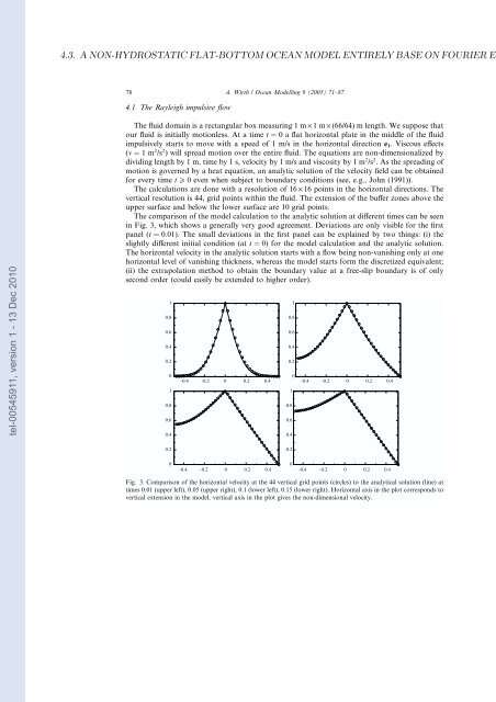
The comparison of the model calculation to the analytic solution at different times can be seen
in Fig. 3, which shows a generally very good agreement. Deviations are only visible for the first
panel (t ¼ 0:01). The small deviations in the first panel can be explained by two things: (i) the
slightly different initial condition (at t ¼ 0) for the model calculation and the analytic solution.
The horizontal velocity in the analytic solution starts with a flow being non-vanishing only at one
horizontal level of vanishing thickness, whereas the model starts form the discretized equivalent;
(ii) the extrapolation method to obtain the boundary value at a free-slip boundary is of only
second order (could easily be extended to higher order).
1
0.8
0.6
0.4
0.2
0
1
0.8
0.6
0.4
-0.4 -0.2 0 0.2 0.4
1
0.8
0.6
0.4
0.2
1
0.8
0.6
0.4
0
-0.4 -0.2 0 0.2 0.4
0.2
0.2
0
-0.4 -0.2 0 0.2 0.4
0
-0.4 -0.2 0 0.2 0.4
Fig. 3. Comparison of the horizontal velocity at the 44 vertical grid points (circles) to the analytical solution (line) at
times 0.01 (upper left), 0.05 (upper right), 0.1 (lower left), 0.15 (lower right). Horizontal axis in the plot corresponds to
vertical extension in the model, vertical axis in the plot gives the non-dimensional velocity.