Ensaios Econômicos - Sistema de Bibliotecas da FGV - Fundação ...

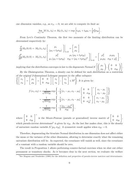
one dimension vanishes, e.g., as 11 ! 0, we are able to compute its limit as:
lim M (t 1; t 2 ) M 2 (t 1 ; t 2 ) = exp
t 1 1 + t 2 2 + 1
11 !0 2 t2 2 22 :
From Levi’s Continuity Theorem, the …rst two moments of the limiting distribution can be
determined respectively by:
"
# " #
d
dt M t=0
1
1
2 (0; 0) = M 2 (t 1 ; t 2 )
=
( 2 + t 2 22 )
2
"
# "
#
d 2
dt 2 M 2 1 1 ( 2 + t 2 22 ) t=0
2 1 1 2
2 (0; 0) = M 2 (t 1 ; t 2 )
1 ( 2 + t 2 22 ) 22 + ( 2 + t 2 22 ) 2 =
1 2 22 + 2 ;
2
" !
!#
1 0 0
implying that the distribution converges in law to the degenerate Normal N ;
.
2 0 22
By the Disintegration Theorem, a density can be de…ned for such distribution on a restriction
of (" the original # " 2-dimensional " Lebesgue measure " to the a¢ ne subspace
x 1
=
x 2
#
1
+
2
f (x 1 ; x 2 ) =
=
=
# "
0 0
0 22
#
v 1
:
v 2
(
1
p exp 222
(
1
p exp 222
(
1
p exp 222
#
v 1
2 R
). 2 It is given by:
v 2
"
1
2 [x 1 1 ; x 2 2 ]
1
2 [x 1 1 ; x 2 2 ]
)
1 [x 2 2 ] 2
;
2 22
"
# + "
0 0
0 22
0 0
0 1
22
# "
#)
x 1 1
x 2 2
#)
x 1 1
x 2 2
" # + " #
0 0
0 0
where
is the Moore-Penrose (pseudo or generalized) inverse matrix of
,
0 22 0 22
which pseudo-inverse determinant 5 is given by 22 . As the last line makes clear, this is the density
of univariate random variable N [ 2 ; 22 ]. A symmetric result applies when 22 ! 0.
Therefore, degenerating the bivariate Normal distribution in one dimension does not a¤ect either
the mean or the variance of the other dimension, allowing to determine exactly what the remaining
univariate distribution will be. As expected, the covariance will vanish as well, since the covariance
of a constant with a random variable should be zero.
The result in Proposition 1 allows performing counter-factual exercises when we shut out either
permanent or transitory shocks. As it becomes clear in the next section, we evaluate the welfare
5 See Magnus and Neudecker (1988) for the de…nition and properties of pseudo-inverse matrices and determinants.
9