Ensaios Econômicos - Sistema de Bibliotecas da FGV - Fundação ...

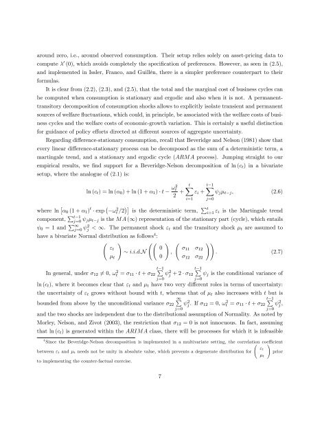
around zero, i.e., around observed consumption. Their setup relies solely on asset-pricing data to
compute 0 (0), which avoids completely the speci…cation of preferences. However, as seen in (2.5),
and implemented in Issler, Franco, and Guillén, there is a simpler preference counterpart to their
formulas.
It is clear from (2.2), (2.3), and (2.5), that the total and the marginal cost of business cycles can
be computed when consumption is stationary and ergodic and also when it is not. A permanenttransitory
decomposition of consumption shocks allows to explicitly isolate transient and permanent
sources of welfare ‡uctuations, which could, in principle, be associated with the welfare costs of business
cycles and the welfare costs of economic-growth variation. This is certainly a useful distinction
for guidance of policy e¤orts directed at di¤erent sources of aggregate uncertainty.
Regarding di¤erence-stationary consumption, recall that Beveridge and Nelson (1981) show that
every linear di¤erence-stationary process can be decomposed as the sum of a deterministic term, a
martingale trend, and a stationary and ergodic cycle (ARMA process). Jumping straight to our
empirical results, we …nd support for a Beveridge-Nelson decomposition of ln (c t ) in a bivariate
setup, where the analogue of (2.1) is:
ln (c t ) = ln ( 0 ) + ln (1 + 1 ) t
tX
2 + Xt 1
" i +
! 2 t
i=1
j=0
j t j ; (2.6)
where ln 0 (1 + 1 ) t exp ! t 2 =2 is the deterministic term, P t
i=1 " i is the Martingale trend
component, P t 1
j=0 j t j is the MA (1) representation of the stationary part (cycle), which entails
0 = 1 and P 1
j=0 j 2 < 1. The permanent shock " t and the transitory shock t are assumed to
have a bivariate Normal distribution as follows 4 :
!
" t
i:i:d:N
t
In general, under 12 6= 0, ! t 2 tP
1
= 11 t + 22
0
0
j=0
!
2
;
j + 2 12
!!
11 12
: (2.7)
12 22
tP
1
j=0
j is the conditional variance of
ln (c t ), where it becomes clear that " t and t have two very di¤erent roles in terms of uncertainty:
the uncertainty of " t grows without bound with t, whereas that of t also increases with t but is
1P
bounded from above by the unconditional variance
2 22 j . If 12 = 0, ! t 2 tP
1
= 11 t +
2 22 j ,
and the two shocks are independent due to the distributional assumption of Normality. As noted by
Morley, Nelson, and Zivot (2003), the restriction that 12 = 0 is not innocuous. In fact, assuming
that ln (c t ) is generated within the ARIMA class, there will be processes for which it is infeasible
4 Since the Beveridge-Nelson decomposition is implemented in a multivariate setting, the correlation coe¢ ! cient
" t
between " t and t needs not be unity in absolute value, which prevents a degenerate distribution for prior
t
to implementing the counter-factual exercise.
j=0
j=0
7