Ensaios Econômicos - Sistema de Bibliotecas da FGV - Fundação ...

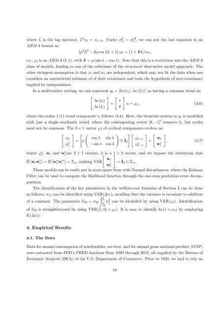
where L is the lag operator, L k x t = x t
ARMA format as:
i.e., ' t is an ARMA (2; 1), with = (sin
k . Under 2 w = 2
w , we can put the last equation in an
2 L 2 2 cos L + 1 ' t = (1 + L) w t ;
cos ). Note that this is a restriction into the ARMA
class of models, leading to one of the criticisms of the structural time-series model approach. The
other stringent assumption is that t and w t are independent, which may not …t the data when one
considers an unrestricted estimate of of their covariance and tests the hypothesis of zero covariance
implied by independence.
In a multivariate setting, we can represent y t = (ln (c t ) ; ln (I t )) 0 as having a common trend as:
" # " #
ln (c t ) 1
= t + ' t ; (3.6)
ln (I t )
where the scalar I (1) trend component t follows (3.4). Here, the bivariate system in y t is modelled
with just a single stochastic trend, where the cointegrating vector [;
1] 0 removes it, but cycles
need not be common. The 2 1 vector ' t of cyclical components evolves as:
" # "
! # " # " #
' t
cos sin
' t 1 w t
=
I 2 + ; (3.7)
sin cos
' t
where ' t , w t and wt are 2 1 vectors, "
is a 1#
2 vector, and we impose the restriction that
E (w t w 0 t) = E (w t w 0
t ) = ! , making VAR
w t
w t
= I 2 ! .
These models can be easily put in state-space form with Normal disturbances, where the Kalman
Filter can be used to compute the likelihood function through the one-step prediction error decomposition.
The identi…cation of the key parameters in the welfare-cost formulas of Section 2 can be done
as follows: 11 can be identi…ed using VAR( t ), recalling that the variance is invariant to addition
1P
of a constant. The parameter e 22 =
2 22 j can be identi…ed by using VAR(' t). Identi…cation
j=0
of e 22 is straightforward by using VAR([1; 0] ' t ). It is easy to identify ln (1 + 1 ) by employing
E ( t ).
' t 1
w t
4. Empirical Results
4.1. The Data
Data for annual consumption of nondurables, services, and for annual gross national product (GNP)
were extracted from FED’s FRED database from 1929 through 2012, all supplied by the Bureau of
Economic Analysis (BEA) of the U.S. Department of Commerce. Prior to 1929, we had to rely on
18