Anisotropic Delaunay Mesh Adaptation for Unsteady Simulations

More documents

Recommendations

Info

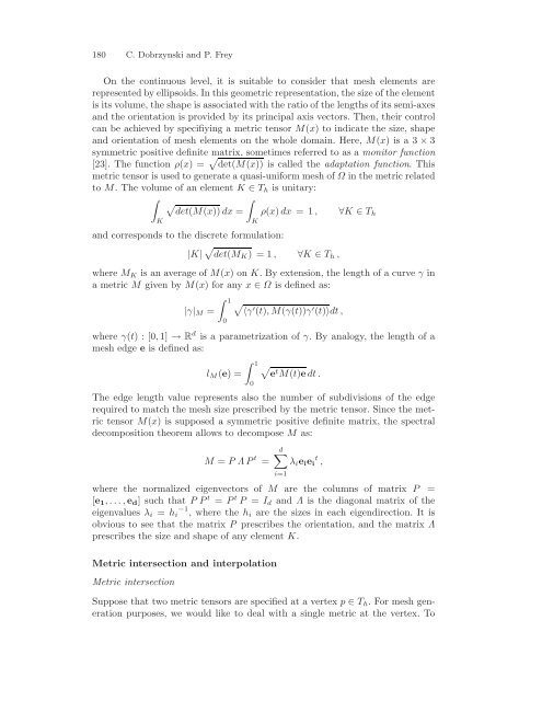
180 C. Dobrzynski and P. Frey On the continuous level, it is suitable to consider that mesh elements are represented by ellipsoids. In this geometric representation, the size of the element is its volume, the shape is associated with the ratio of the lengths of its semi-axes and the orientation is provided by its principal axis vectors. Then, their control can be achieved by specifiying a metric tensor M(x) to indicate the size, shape and orientation of mesh elements on the whole domain. Here, M(x) isa3 × 3 symmetric positive definite matrix, sometimes referred to as a monitor function [23]. The function ρ(x) = √ det(M(x)) is called the adaptation function. This metric tensor is used to generate a quasi-uniform mesh of Ω in the metric related to M. The volume of an element K ∈ T h isunitary: ∫ √ ∫ det(M(x)) dx = ρ(x) dx =1, ∀K ∈ T h K and corresponds to the discrete formulation: K |K| √ det(M K ) = 1 , ∀K ∈ T h , where M K isan average of M(x) on K. By extension, the length of a curve γ in a metric M given by M(x) for any x ∈ Ω is defined as: |γ| M = ∫ 1 0 √ 〈γ′ (t),M(γ(t))γ ′ (t)〉dt , where γ(t) : [0, 1] → R d is a parametrization of γ. By analogy, the length of a mesh edge e is defined as: l M (e) = ∫ 1 0 √ et M(t)e dt . The edge length value represents also the number of subdivisions of the edge required to match the mesh size prescribed by the metric tensor. Since the metric tensor M(x) is supposed a symmetric positive definite matrix, the spectral decomposition theorem allows to decompose M as: M = P Λ P t = d∑ λ i e i e t i , where the normalized eigenvectors of M are the columns of matrix P = [e 1 ,...,e d ] such that PP t = P t P = I d and Λ is the diagonal matrix of the eigenvalues λ i = h i −1 ,where the h i are the sizes in each eigendirection. It is obvious to see that the matrix P prescribes the orientation, and the matrix Λ prescribes the size and shape of any element K. Metric intersection and interpolation Metric intersection Suppose that two metric tensors are specified at a vertex p ∈ T h . For mesh generation purposes, we would like to deal with a single metric at the vertex. To i=1
Anisotropic Delaunay Mesh Adaptation for Unsteady Simulations 181 this end, we define a metric intersection procedure. Geometrically speaking, it consists in defining the largest ellipsoid E included in the intersection of the two ellipsoids E 1 and E 2 associated with the two metric tensors. From the algebraic point of view, we use the simutaneous reduction of the two underlying quadratic forms to find a basis of the vector space in which the matrices M and N associated with E 1 and E 2 are represented respectively by I 3 and D, adiagonal matrix of M 3 (R). Denoting by P = ( e 1 e 2 e 3 ) the invertible matrix of GL3 (R) formed by the eigenvectors e i ,i=1, 3of the matrix N ′ = M −1 N leads to define the intersection matrix M ∩ as: M ∩ =(P t ) −1 ΛP −1 ,where Λ is the diagonal matrix with the coefficients max(λ i ,µ i ). Metric interpolation Consider a parametrization of a mesh edge pq as c : [0, 1] → R 3 , c(t) = (1−t)p+tq andtwo metric tensors M p and M q associated with the endpoints.We are looking for the metric tensor at t, hence for a matrix M(t) defined along the segment c(t) for any value of the parameter t ∈ [0, 1]. The definition of this matrix M(t) involves the interpolation of the eigenvalues of the matrices M p and M q .This procedure allows one to define acontinuous metric field along the segment. To this end, we suggest the following linear interpolation scheme: M(t) = ( ) (1 − t)M − 1 2 p + tM − 1 −2 2 q , 0 ≤ t ≤ 1 . (1) Finding the interpolated metric tensor M t requires us to express the two matrices in a basis {e i } in which both are congruent to adiagonal matrix and then to deduce the metric tensor at point t. In other words, this scheme is similar to reducing simultaneously the two quadratic forms associated with the metrics. 2.3 Mesh Quality Measures There are several reasons for assessing a mesh and controlling its quality. In particular, it is useful to know if the mesh elements are aligned with the physical solution, especially in the anisotropic context. Then, in the adaptive context, it is important to know how closely the equiditribution and alignment conditions are satisfied by the mesh. Finally, in three dimensions, a quasi-uniform mesh is not easy to produce if only controlling the lengths of mesh edges. It is well known that slivers (null volume) elements may occur and their creation cannot be prevented by simply checking the their edge lengths. The topics of mesh quality and mesh assessment have been studied in the context of finite element methods in numerous papers. We refer the reader to [2] and the references therein for more details on the related issues. Classicalquality measures include minimal angle condition [35] or maximal angle condition [4] as well as aspect ratio considerations. Other works include error estimates to account for the shape of the element and the solution behavior [6]. The adequacy
Page 1 and 2: Anisotropic Delaunay Mesh Adaptatio
Page 3: Anisotropic Delaunay Mesh Adaptatio

Anisotropic Delaunay Mesh Adaptation for Unsteady Simulations

Create successful ePaper yourself

Delete template?

Save as template?