Anisotropic Delaunay Mesh Adaptation for Unsteady Simulations

182 C. Dobrzynski and P. Frey
between anisotropicelements and the anisotropyof the solution can be measured
by a matching function [25].
Given a metric tensor field M(x), it is natural to define critera to measure how
closely the mesh elements are aligned and equidistributed with respect to M(x).
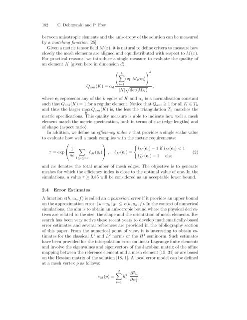
For practical reasons, we introduce a single measure to evaluate the quality of
an element K (given here in dimension d):
〈e i ,M K e i 〉
( k∑
i=1
Q ani (K) =α d
|K| √ det(M K )
where e i represents any of the k egdes of K and α d isanormalisation constant
such that Q ani (K) = 1 for a regular element. Notice that Q ani ≥ 1 forall K ∈ T h
and thus the larger max Q ani(K) is, the less the triangulation T h matches the
K
metric specifications. This quality measure is able to indicate how well a mesh
element match the metric specification, both in terms of size (edge lengths) and
of shape (aspect ratio).
In addition, we define an efficiency index τ that provides a single scalar value
to evaluate how well a mesh complies with the metric requirements:
⎛
⎞
{
∑
lM (e i ) − 1if l M (e i ) < 1
τ = exp ⎝ 1 ne
1≤i≤ne
l M (e i ) ⎠ , l M (e i )=
) d
,
l −1
M (e i) − 1
and ne denotes the total number of mesh edges. The objective is to generate
meshes for which the efficiency index isclose to the optimal value of one. In the
simulations, a value τ ≥ 0.85 will be considered as an acceptable lower bound.
else
(2)
2.4 Error Estimates
A function e(h, u h ,f)is called an a posteriori error if it provides an upper bound
on the approximation error: ‖u−u h ‖ W ≤ e(h, u h ,f). In the context of numerical
simulations, the aim is toobtain an anisotropic bound where the physical derivatives
are related to the size, the shape and the orientation of mesh elements. Research
has been very active these recent years to develop mathematically-based
error estimates and several references are provided in the bibliography section
of this paper. From the numerical point of view, it is interesting toobtain estimates
for the classical L 1 and L 2 norms or the H 1 seminorm. Such estimates
have been provided for the interpolation error on linear Lagrange finite elements
and involve the eigenvalues and eigenvectors of the Jacobian matrix of the affine
mapping between the reference element and a mesh element [15, 31] or are based
on the Hessian matrix of the solution [18, 1]. A local error model can be defined
at a mesh vertex p as follows:
e M (p) =
d∑
i=1
h 2 i
∂ 2 u
∣ ∣ ,
∂α 2 i