Download - ASLO

1772
Notes
J
1.0
2
E 0.9
L
2 0.6
P
< 0.7
t 0.6
0.010
1 10 100
Velocity, cm s-1
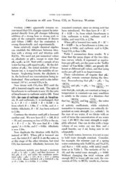
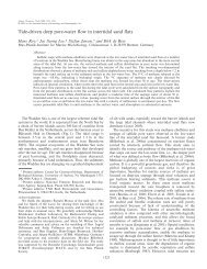
Fig. 3. Plot ofclod card weight loss vs. velocity through
32o/oo seawater for data from Glenn and Doty (1992) used
in the form of Eq. 3 (their data extend to higher velocities
than our work). The slope of the regression line is
0.838kO.042.
0.5
0.4 r I
0 5 10 15 20 25 30
Temperature, "C
Fig. 4. Correction factor for clod card data with T,, =
298°K and pref = viscosity of pure water at 25°C. The four
lines correspond to salinities of 0, 10, 20, and 40%~ from
top to bottom. Calculated with viscosity data from Riley
and Skit-row (1975).
(e.g., Cussler 1984; Sherwood et al. 1975; Skelland
1974). For solids of sample geometries
which dissolve uniformly, the area and weight
relationship can be approximated as
A (2)
Ai and Wi represent the initial area (exposed)
and weight of the solid. For clod cards, this
approximation is useful until > 50% of the clod
has dissolved or longer, depending on the velocity
of the fluid.
The mass transfer coefficient is also influenced
by the change in clod dimensions; however,
the effect is usually minor until well into
the dissolution process. Equations 1 and 2 can
be combined and integrated to give
1 - (?r = ;k($A,. (3)
Wr is the final weight of the clod after time 8
has elapsed. Equations 3 is useful for data analysis;
the mass transfer coefficient usually varies
with the fluid velocity raised to a power (P),
so a log-log plot of [l - (WJ/ Wi)“] against
velocity should yield a straight line. This is
illustrated in Fig. 3 with the data of Glenn and
Doty (1992). Equation 3 can be rearranged to
give an expression for the overall fraction of
weight 10~s (A W/ Wi):
Assuming that AC remained constant during
dissolution, experimental data at a given temperature
and salinity were correlated with the
model
( )
l/3
Wf = aVm.
I- j7
I
The constants a and m can be determined experimentally
by means of the rotating arm, and
weight loss data from clod cards exposed in
the field can then be used in Eq. 5 to determine
water motion.
The effect of temperature at a given salinity
and CaSO, concentration was corrected by using
the group (T/T,,) (p,.,&) to normalize data
to a reference temperature, where Tis absolute
temperature, and p is viscosity. This group (Fig.
4) is typically used to estimate the changes in
diffusion coefficients (Reid and Sherwood
1966) with varying solution strength.
From Eq. 1 and 3, the dissolution rates are
also dependent on the concentration of CaSO,
in the bulk water and factors influencing the
concentration, such as the ionic strength of the
bulk water. To determine the concentration
difference, we assume the solution at the gypsum-water
interface is saturated with CaSO,
and determine AC with the solubility product
as
Ksp = [Ca2+]i[S042-]i
g= 1 - 11 - ;k($)ACO13. (4)
or
= ([Ca’+], + AC)([S042-]b + AC) (6)