∑ ∑

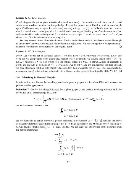
Lemma 5. BM LP is integral.
Proof. Suppose the primal gives a fractional optimal solution x ⋆ e. If we can find a cycle, then one of e’s end
vertex must also have another non-integral edge. Repeat this process we will end up with an even length
cycle C with non-integral edges. Let ∆ = min(min e∈C x ⋆ e,min e∈C (1 − x ⋆ e)), and x ′ be the same as x ⋆ except
that ∆ is added to the odd edges and −∆ is added to the even edges. Similarly, let x ′′ be the same as x ⋆ but
with −∆ is added to the odd edges and ∆ is added to the even edges. It should be noted that x ⋆ = x ′ = x ′′ , so
either x ′ or x ′′ has introduced at least an integral x e .
We may also find a tree of fractional values. Similar to the above analysis, we choose a ∆ small enough
so that none of the constraints become violated after the adjustment. We can average these “complementary”
solutions to contradict the extremity of the original point.
Lemma 6. VC LP is integral.
Proof. Let F be the set of fractional vertices. We must have F ≠ /0; otherwise we are done. Let U and
V be the two components of the graph and, without loss of generality, we assume that |F ∩U| ≥ |F ∩V |.
Let ∆ = min{y ⋆ v|v ∈ F ∩U}, in which y ⋆ v is the optimal solution to VC LP . Subtract ∆ from all elements in
F ∩U and add ∆ to all elements in F ∩V . By doing so we do not violate any constraint of the dual, instead,
we have obtained a solution with objective function less than or equal to the original. This contradicts the
assumption that y ⋆ v is the optimal solution to VC LP . Hence, we have proved the integrality of the VC LP.
3.4 Matching in General Graphs
In this section, we discuss the matching problem in general graphs and introduce Edmonds’ theorem on
perfect matching polytopes.
Definition 7. (Perfect Matching Polytope) For a given graph G, the perfect matching polytope M is the
covex hull of all the matchings in G, thus
{
}
P(G) =
∑
i
As we have seen, the constraints
λ i M i |∀i λ i ≥ 0,M i per f ect matching in G, and∑λ i = 1
i
∑
e∈E v
x e ≤ 1,∀v ∈ V
x e ≥ 0,∀e ∈ E
are not sufficient to define correctly a perfect matching. For example, E = { 1
2 , 1 2 , 2} 1 satisfies the above
constraints while these edges form a triangle. Let S ⊆ V be an odd size set and M be any perfect matching of
G. One must see that at most 1 2
(|S| − 1) edges inside S. We can adapt this observation to the linear program
for perfect matchings:
max ∑ x e
e∈E
s.t. ∑
x e ≤ 1, ∀v ∈ V
e∈E v
⌊ |S|
∑ x e ≤
2
e∈E(S)
x e ≥ 0, ∀e ∈ E
⌋
, ∀v ∈ V
9-4