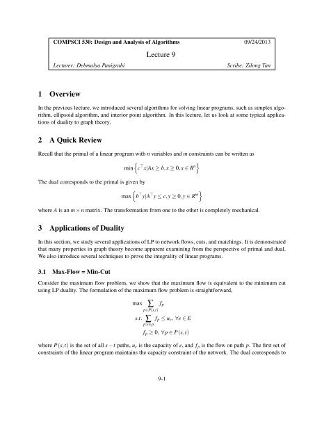
∑ ∑

COMPSCI 530: Design and Analysis of Algorithms 09/24/2013
Lecturer: Debmalya Panigrahi
Lecture 9
Scribe: Zilong Tan
1 Overview
In the previous lecture, we introduced several algorithms for solving linear programs, such as simplex algorithm,
ellipsoid algorithm, and interior point algorithm. In this lecture, let us look at some typical applications
of duality to graph theory.
2 A Quick Review
Recall that the primal of a linear program with n variables and m constraints can be written as
min
{c ⊤ x|Ax ≥ b,x ≥ 0,x ∈ R n}
The dual corresponds to the primal is given by
max
{b ⊤ y|A ⊤ y ≤ c,y ≥ 0,y ∈ R m}
where A is an m × n matrix. The transformation from one to the other is completely mechanical.
3 Applications of Duality
In this section, we study several applications of LP to network flows, cuts, and matchings. It is demonstrated
that many properties in graph theory become apparent examining from the perspective of primal and dual.
We also introduce several techniques to prove the integrality of linear programs.
3.1 Max-Flow = Min-Cut
Consider the maximum flow problem, we show that the maximum flow is equivalent to the minimum cut
using LP duality. The formulation of the maximum flow problem is straightforward,
max
∑
p∈P(s,t)
f p
s.t. ∑ f p ≤ u e , ∀e ∈ E
p:e∈p
f p ≥ 0, ∀p ∈ P(s,t)
where P(s,t) is the set of all s −t paths, u e is the capacity of e, and f p is the flow on path p. The first set of
constraints of the linear program maintains the capacity constraint of the network. The dual corresponds to
9-1

the primal follows
min ∑ u e l e
e∈E
s.t. ∑ l e ≥ 1, ∀p ∈ P(s,t)
e:e∈p
l e ≥ 0, ∀e ∈ E
where l e can be interpreted as the length of the edge e in OPT D and u e l e therefore corresponds to the volume
of the edge. So the objective of the dual is to find the volume-minimizing assignment of lengths to the edges
so that that every s −t path has length at least 1.
Theorem 1. Max-flow = Min-cut.
Proof. First, we show that the dual above has 0−1 basic feasible solution. For an s−t cut ( S,S ) , let E ( S,S )
denote the edges crossing the cut and let u ( S,S ) denote the sum of capacities of edges crossing the cut. For
any s −t cut ( S,S ) , let l e = 1 for all e ∈ E ( S,S ) and l e = 0 for all others. Clearly, this is a feasible solution
for the dual. It follows from weak duality theorem, max-flow ≤ OPT D ≤ integral min-cut.
Next, we prove the other direction. Let l e be the length function and let d (v) be the shortest distance
from s to v for all v ∈ V according to the lengths l e . Note that d (s) = 0 and d (t) ≥ 1. Consider ρ ∈ U.A.R [0,1)
and let S ρ = {v ∈ V |d (v) ≤ ρ}, it follows
E [ u ( )]
S ρ ,S ρ = ∑ u e Pr ( e ∈ E ( ))
S ρ ,S ρ
e∈E
Note that Pr ( e ∈ E ( S ρ ,S ρ
))
≤ le , we obtain
E [ u ( )]
S ρ ,S ρ ≤ ∑ u e l e
e∈E
This implies that there exists a ρ with u ( )
S ρ ,S ρ ≤ ∑e∈E u e l e , i.e. min-cut ≤ OPT D , which proves that maxflow
= min-cut by strong duality theorem. Observe that for any u e ’s, there exists an integer s−t cut ( )
S ξ ,S ξ
with cost at most ∑ e∈E u e l e . This cut corresponds to
{1 e ∈ E ( )
S ξ ,S ξ
y e =
0 otherwise
Clearly, y is also feasible for the dual. Now we have ∑ e∈E u e y e ≤ OPT D , it follows that ∑ e∈E u e y e = OPT D
and l e = y e in OPT D . Thus, we have proved the integrality of l e ’s.
3.2 Global Min-Cut
Let us then consider the global min-cut problem. We show how to formulate a linear program and its dual
for the global min-cut problem. The definition of the global min-cut problem is given as follows.
Definition 2. (Global Min-Cut) Given in input an undirected graph G = (V,E) we want to find the subset
A ⊆ V such that A ≠ /0, A ≠ V , and the number of edges with one endpoint in A and one endpoint in V − A
is minimized.
9-2

The basic intuition behind is that for any spanning tree of the graph, at least one of its edge must be
included in the cut. Since if not, the graph remains connected after the cut. The linear program for a global
min-cut problem follows
min
e∈E x e
s.t. ∑ x e ≥ 1, ∀spanningtree T
e∈T
x e ≥ 0,∀e ∈ E
where x e ∈ [0,1] is the variable associated with edge e, indicating whether e is included in the min-cut. The
dual corresponds to the primal is written as
max∑y T
T
s.t. ∑ y T ≤ 1, ∀e ∈ E
T :e∈T
y T ≥ 0, ∀T
It should be noted that these linear programs are not integral.
3.3 Bipartite Matching
In this section, we show that the maximum bipartite matching is equal to the minimum vertex cover using
the primal and dual. The definition of a matching is given as follows.
Definition 3. A matching is a set of edges which do not intersect at any vertices.
Theorem 4. (König’s Theorem [1]) Given a bipartite graph G = (V,E), let C be a vertex cover in G and M
be a matching in G, then min|C| = max|M|.
Proof. Let BM and BM LP denote the cardinality of the maximum matching and the optimal value of the
maximum matching LP relaxation, we have that BM LP is given by
max ∑ x e
e∈E
s.t. ∑ x e ≤ 1, ∀v ∈ V
e∈E v
x e ≥ 0, ∀e ∈ E
where E v represents the set of edges incident on vertex v. The dual for the primal then follows
min ∑ y v
v∈V
s.t.y u + y v ≥ 1, ∀(u,v) ∈ E
y v ≥ 0, ∀v ∈ V
Let VC and VC LP denote the cardinality of the minimum vertex cover, and the optimal value of the vertex
cover LP relaxation, respectively. The dual is the linear program for finding VC LP . Enforcing the integrality
constraint of the dual gives us VC. It follows from duality theory,
BM ≤ BM LP = VC LP ≤ VC
The following lemmas prove the integrality of BM LP and VC LP , hence we have BM = VC.
9-3

Lemma 5. BM LP is integral.
Proof. Suppose the primal gives a fractional optimal solution x ⋆ e. If we can find a cycle, then one of e’s end
vertex must also have another non-integral edge. Repeat this process we will end up with an even length
cycle C with non-integral edges. Let ∆ = min(min e∈C x ⋆ e,min e∈C (1 − x ⋆ e)), and x ′ be the same as x ⋆ except
that ∆ is added to the odd edges and −∆ is added to the even edges. Similarly, let x ′′ be the same as x ⋆ but
with −∆ is added to the odd edges and ∆ is added to the even edges. It should be noted that x ⋆ = x ′ = x ′′ , so
either x ′ or x ′′ has introduced at least an integral x e .
We may also find a tree of fractional values. Similar to the above analysis, we choose a ∆ small enough
so that none of the constraints become violated after the adjustment. We can average these “complementary”
solutions to contradict the extremity of the original point.
Lemma 6. VC LP is integral.
Proof. Let F be the set of fractional vertices. We must have F ≠ /0; otherwise we are done. Let U and
V be the two components of the graph and, without loss of generality, we assume that |F ∩U| ≥ |F ∩V |.
Let ∆ = min{y ⋆ v|v ∈ F ∩U}, in which y ⋆ v is the optimal solution to VC LP . Subtract ∆ from all elements in
F ∩U and add ∆ to all elements in F ∩V . By doing so we do not violate any constraint of the dual, instead,
we have obtained a solution with objective function less than or equal to the original. This contradicts the
assumption that y ⋆ v is the optimal solution to VC LP . Hence, we have proved the integrality of the VC LP.
3.4 Matching in General Graphs
In this section, we discuss the matching problem in general graphs and introduce Edmonds’ theorem on
perfect matching polytopes.
Definition 7. (Perfect Matching Polytope) For a given graph G, the perfect matching polytope M is the
covex hull of all the matchings in G, thus
{
}
P(G) =
∑
i
As we have seen, the constraints
λ i M i |∀i λ i ≥ 0,M i per f ect matching in G, and∑λ i = 1
i
∑
e∈E v
x e ≤ 1,∀v ∈ V
x e ≥ 0,∀e ∈ E
are not sufficient to define correctly a perfect matching. For example, E = { 1
2 , 1 2 , 2} 1 satisfies the above
constraints while these edges form a triangle. Let S ⊆ V be an odd size set and M be any perfect matching of
G. One must see that at most 1 2
(|S| − 1) edges inside S. We can adapt this observation to the linear program
for perfect matchings:
max ∑ x e
e∈E
s.t. ∑
x e ≤ 1, ∀v ∈ V
e∈E v
⌊ |S|
∑ x e ≤
2
e∈E(S)
x e ≥ 0, ∀e ∈ E
⌋
, ∀v ∈ V
9-4

Here, E (S) is the set of edges induced by S. Edmonds proved that the above LP corresponds to the perfect
matching P(G) in G, and is integral [2].
4 Summary
In this lecture, we discussed several typical applications of duality to graph theory. First, we formulated
the linear programs and the duals for the these problems. Next, the duality theory was used to establish
a connection between the primal objective function and the dual objective function. We also proved the
integrality of the primal and dual linear programs.
References
[1] http://en.wikipedia.org/wiki/K%C3%B6nig%27s theorem %28graph theory%29
[2] J. Edmonds, Maximum matching and a polyhedron with 0, 1-vertices,J. Res. Nat. Bur. Standards Sect.
B 69 (1965) 125–130.
9-5