Sharing the Cost of Backbone Networks - Computer Science

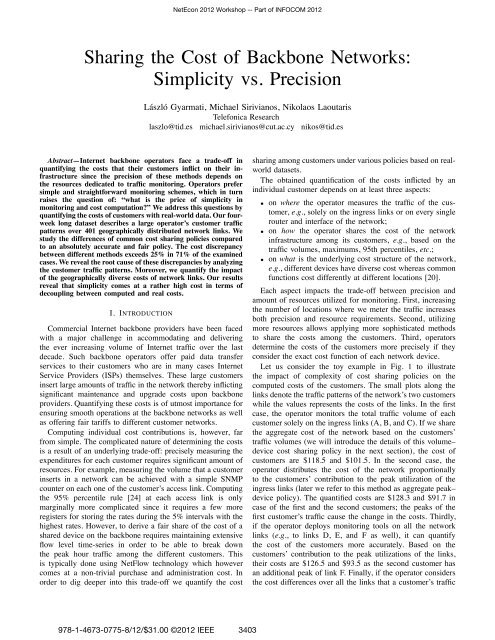
NetEcon 2012 Workshop -- Part of INFOCOM 2012
Sharing the Cost of Backbone Networks:
Simplicity vs. Precision
László Gyarmati, Michael Sirivianos, Nikolaos Laoutaris
Telefonica Research
laszlo@tid.es michael.sirivianos@cut.ac.cy nikos@tid.es
Abstract—Internet backbone operators face a trade-off in
quantifying the costs that their customers inflict on their infrastructure
since the precision of these methods depends on
the resources dedicated to traffic monitoring. Operators prefer
simple and straightforward monitoring schemes, which in turn
raises the question of: “what is the price of simplicity in
monitoring and cost computation?” We address this questions by
quantifying the costs of customers with real-world data. Ourfourweek
long dataset describes a large operator’s customer traffic
patterns over 401 geographically distributed network links. We
study the differences of common cost sharing policies compared
to an absolutely accurate and fair policy. The cost discrepancy
between different methods exceeds 25% in 71% of the examined
cases. We reveal the root cause of these discrepancies by analyzing
the customer traffic patterns. Moreover, we quantify the impact
of the geographically diverse costs of network links. Our results
reveal that simplicity comes at a rather high cost in terms of
decoupling between computed and real costs.
I. INTRODUCTION
Commercial Internet backbone providers have been faced
with a major challenge in accommodating and delivering
the ever increasing volume of Internet traffic over the last
decade. Such backbone operators offer paid data transfer
services to their customers who are in many cases Internet
Service Providers (ISPs) themselves. These large customers
insert large amounts of traffic in the network thereby inflicting
significant maintenance and upgrade costs upon backbone
providers. Quantifying these costs is of utmost importance for
ensuring smooth operations at the backbone networks as well
as offering fair tariffs to different customer networks.
Computing individual cost contributions is, however, far
from simple. The complicated nature of determining the costs
is a result of an underlying trade-off: precisely measuring the
expenditures for each customer requires significant amount of
resources. For example, measuring the volume that a customer
inserts in a network can be achieved with a simple SNMP
counter on each one of the customer’s access link. Computing
the 95% percentile rule [24] at each access link is only
marginally more complicated since it requires a few more
registers for storing the rates during the 5% intervals with the
highest rates. However, to derive a fair share of the cost of a
shared device on the backbone requires maintaining extensive
flow level time-series in order to be able to break down
the peak hour traffic among the different customers. This
is typically done using NetFlow technology which however
comes at a non-trivial purchase and administration cost. In
order to dig deeper into this trade-off we quantify the cost
sharing among customers under various policies based on realworld
datasets.
The obtained quantification of the costs inflicted by an
individual customer depends on at least three aspects:
• on where the operator measures the traffic of the customer,
e.g., solelyontheingresslinksoroneverysingle
router and interface of the network;
• on how the operator shares the cost of the network
infrastructure among its customers, e.g., basedonthe
traffic volumes, maximums, 95th percentiles, etc.;
• on what is the underlying cost structure of the network,
e.g., differentdeviceshavediversecostwhereascommon
functions cost differently at different locations [20].
Each aspect impacts the trade-off between precision and
amount of resources utilized for monitoring. First, increasing
the number of locations where we meter the traffic increases
both precision and resource requirements. Second, utilizing
more resources allows applying more sophisticated methods
to share the costs among the customers. Third, operators
determine the costs of the customers more precisely if they
consider the exact cost function of each network device.
Let us consider the toy example in Fig. 1 to illustrate
the impact of complexity of cost sharing policies on the
computed costs of the customers. The small plots along the
links denote the traffic patterns of the network’s two customers
while the values represents the costs of the links. In the first
case, the operator monitors the total traffic volume of each
customer solely on the ingress links (A, B, and C). If we share
the aggregate cost of the network based on the customers’
traffic volumes (we will introduce the details of this volume–
device cost sharing policy in the next section), the cost of
customers are $118.5 and $101.5. In the second case, the
operator distributes the cost of the network proportionally
to the customers’ contribution to the peak utilization of the
ingress links (later we refer to this method as aggregate peak–
device policy). The quantified costs are $128.3 and $91.7 in
case of the first and the second customers; the peaks of the
first customer’s traffic cause the change in the costs. Thirdly,
if the operator deploys monitoring tools on all the network
links (e.g., tolinksD,E,andFaswell),itcanquantify
the cost of the customers more accurately. Based on the
customers’ contribution to the peak utilizations of the links,
their costs are $126.5 and $93.5 as the second customer has
an additional peak of link F. Finally, if the operator considers
the cost differences over all the links that a customer’s traffic
978-1-4673-0775-8/12/$31.00 ©2012 IEEE 3403

2
x
200
150
100
50
x
200
150
100
50
1 2
2
x
200
150
100
50
10$
1
t
A
t
1
2
10$
t
20$
D
B
x
200
150
100
50
50$
F
100$
x
200
150
100
E
2
50
2
t
x
C 200
1 1
30$ 150
Fig. 1. Toy example: diverse complexity and precision of cost sharing
policies. The plots present the traffic volumes of the customers.
traverses, the customers’ costs change to $114.2 and $105.8
because the second customer utilizes more expensive links.
This example shows that the operator captures the costs of
customers with more precision if it utilizes more resources to
meter the network.
Our work makes the following contributions. First, we
quantify the cost of large customers of a backbone operator
using real traffic. Specifically, we utilize a four-week long
dataset from Netflow traffic information of distinct customers
and of 401 geographically distributed network links located
in 9 countries. We observe that discrepancies arise among
different cost sharing mechanisms; the difference among the
costs is more than 25% in 71% of the cases considering the
most precise and the simplest methods. Moreover, in 12% of
the cases simple pricing is off by at least a factor of ×5.
Second, we identify and explain the causes of the discrepancies
by analyzing the traffic patterns of customers with the largest
discrepancies. The main causes behind the discrepancies are
the stepwise cost functions and that the policies do not
consider the contribution of individual customers to all the
local maxima of the aggregate traffic volumes. Third, we
evaluate the impact of differences in the cost structures of
network devices due to geographic location. Different parts
of a backbone network have diverse costs owed to numerous
factors such as energy prices, deployment costs, operational
expenses, or taxation. We quantify the impact of cost diversity
using real data on transit prices and identify additional
discrepancies between the cost policies.
We present our methodology in Section II, where we
introduce five policies for network cost sharing and reveal the
details of the utilized datasets. In Section III we investigate
the discrepancies of the methods based on empirical results.
Afterwards, we review the related work in Section IV. Last,
in Section V we present the conclusions and outline future
research directions.
II. METHODOLOGY
In this section we introduce the details of our methodology,
i.e., how we quantify the trade-off between precision and
resource needs of the cost sharing policies. We do this by
computing the contribution of individual customers to the
aggregate cost of the network. To this end, first we introduce
t
1
100
50
2
t
several methods that share the costs of the network devices
among the customers. Subsequently, we describe the datasets
we use as input parameters.
We quantify the costs of individual customers under the
following general setting. A network consists of various network
devices, such as routers, switches and links. Let L
denote the set of devices of the network and I the set of
customers of the network. Let x l i (t) denote the traffic volume
injected by customer i ∈ I on network device l ∈ L during
the time interval t in [1,T]. Also,letc l denote the cost of
network device l. Thecostofaspecificdevicedependsonthe
maximum amount of traffic that it has to carry during a certain
time interval. Therefore c l is obtained by examining the costs
of a device for various rates (e.g., 1Gbps,10Gbps,etc.) and
taking the smallest device whose capacity covers the offered
traffic under the requested Service Level Agreement. To this
end, we assume that the device costs follow a step function
C : R → R. Thus,thecostofdevicel is
A. Cost Sharing Policies
c l = C(max
t∈T
∑
i∈I
x l i (t)) (1)
Next, we present several policies for sharing the aggregate
cost of the network infrastructure among the customers.
These policies strike different balances between precision
and resource needs, which we discuss in more details after
their formal descriptions. We note that operators of backbone
networks apply some of these policies in practice for pricing
purposes like the 95th percentile and the aggregate peak
policies. In all cases, we first determine the break down of
the cost of a single device among the customers that use it
and then sum over all devices to get the total cost inflicted by
any given customer.
Volume–device. We measure the amount of data that a single
customer sends on the specific network device (e.g., on a single
link) for the whole duration of the time-series. Afterwards,
we share the cost of the device proportionally to the traffic
volumes of the customers using it. Hence, the cost of customer
i for device l is:
∑
c l i = c l ·
∑
j∈I
t∈T xl i (t)
∑t∈T xl j (t) (2)
95th percentile–device. We distribute the cost of the device
proportional to the 95th percentiles [10] of the customers’
traffic that traverses that device. Hence, we quantify the cost
of customer i for device l as:
c l i = cl ·
(
P 95 ...,x
l
i (t − 1),x l i (t),xl i (t +1)...)
∑
j∈I P (
95 ...,x
l
j (t − 1),x l (3)
j (t),xl j (t +1),...)
where P 95 denotes the 95th percentile of the arguments.
95th percentile–customer. We utilize this policy in Section
III-C to illustrate the importance of the granularity of
metering, we study the sharing of the cost of all the network
devices based on the 95th percentile of the customer’s aggregate
traffic. The customer’s aggregate traffic can be measured
at the entry devices of the network, thus it does not require
3404

3
metering deep in the network. The total cost of customer i is:
c i = ∑ ( ∑
c l P 95 ...,
l∈L ·
xl i
∑
(t),...)
l j∈I P ( (4)
95 ...,
∑l∈L xl j (t),...)
Customer peak–device. Under this policy, we share the
expenditure of the network device based on the customers’
maximal usage volumes for the given time interval; i.e., the
cost of customer i in case of network device l is
c l i = cl ·
max t∈T x l i (t)
∑j∈I max t∈T x l j (t) (5)
Aggregate peak–device. Network operators plan the capacity
of the network based on the maximum utilization, i.e., the
capacity of a link is larger than the expected maximum of the
traffic that traverses it. Accordingly, we distribute the cost of
the devices based on the contribution of individual customers
to the peak utilization. Assuming that the peak utilization of
device l happens at time step t m =argmax t
∑j∈I xl j (t), we
allocate the following cost to customer i:
c l i = x l
cl i ·
(t m)
∑
j∈I xl j (t m)
Shapley–device. This policy distributes the cost of a network
device among the customers in a fair way. For example, a
small customer starts sending 1 Gbps traffic on a 10 Gbps
link that a large customer utilizes nearly completely, e.g., by
sending 9.5 Gbps. Due to the traffic of the small customer,
the operator has to upgrade the capacity of the link from 10
Gbps to 40 Gbps to handle the elevated traffic volume. The
expenditure of the upgrade increases the costs of the network,
for which the small customer is mainly responsible. Thus, the
fair cost of the small customer is much larger than its share
computed solely on the small customer’s peak rates. Under
this policy, the cost of each customer is proportional to its
average marginal contribution to the total cost. Particularly, let
us consider all the possible S ⊂ I subsets (coalitions) of the
customers who utilize resources of the network device l. The
cost of coalition S depends on the aggregate traffic volume of
the participants, i.e., itequalstothecostofanetworkdevice
having enough capacity:
v l (S) =C(max
t∈T
(6)
∑
x l j(t)) (7)
j∈S
Based on the v cost function of the coalitions, the
(φ 1 (v),...,φ N (v)) Shapley values describe the fair distribution
of costs in case of the S = I grand coalition—fair in a
way that it satisfies four intuitive fairness criteria [1, 11, 18].
We compute the Shapley value of customer i as
φ i (v l )= 1 ∑ (
v l (S (Π,i)) − v l (S (Π,i) \ i) ) (8)
N!
Π∈S N
where Π is a permutation or arrival order of set N and
S(Π,i) denotes the set of players who arrived no later than i.
Accordingly, we quantify the cost of customer i based on its
Shapley value:
c l i = φ i (v l )
cl · ∑
j∈I φ j(v l )
While we compute the aggregate traffic volumes of the
coalitions, we make an assumption. Namely, we assume that
the routing inside the network is static, i.e., removingsome
traffic from the network device does not affect the traffic
volumes of other customers (e.g., thenetworkdoesnotapply
load balancing mechanisms).
Some of the above formulas determine the expenditures
caused by the customers on a per device basis. We quantify
the aggregate cost of customer i over the whole network as
the sum of the costs caused on each network device that his
traffic utilizes:
c i = ∑ c l i (10)
l∈L
B. Trade-offs of the cost sharing policies
The introduced cost sharing methods make diverse tradeoffs
in terms of computational complexity, amount of necessary
information, and accuracy. We present the policies in an
order according to their properties.
Computational resources. The volume–device policy requires
the least computational resources as it summarizes only the
traffic volumes of the customers. The customer peak–device,
the aggregate peak–device, and the 95th percentile–device
policies have slightly more complexity because of their maximum
and percentile computations. Finally, the Shapley–device
method has the largest complexity as it computes the costs
based on the different sub-coalitions of the customers. For
computational reasons, we consider the 15 largest customer
per network device to quantify the costs based on the Shapley–
device method. On average, these customers cover 94% of the
traffic of the devices.
Necessary information. In terms of the amount of information,
all the methods except the Shapley–device policy are
similarly modest. They utilize single values for the historical
(sum and maximum, respectively) and the current volume
or rate values. Contrary, the Shapley–device policy uses the
whole time-series of traffic volumes to compute the costs.
Accuracy. The Shapley–device policy method has the highest
precision and fairness. The method determines the costs by
considering the time when the customers send the traffic, the
volume and the burstiness of the traffic, the customers’ contribution
to the peak utilization as well as the step cost function
of the devices. The other policies miss at least one of these
resulting lower accuracies. The aggregate peak–device method
takes into account the size of the burst and the contribution
to the peak utilization of the device, however, it considers
only a single point of time. Accordingly, this policy misses
the information about how much the customer contributes
to the other local maxima of the device’s utilization. The
95th percentile–device policy includes the impact of bursts
and captures the traffic volumes over multiple time intervals.
However, it does not reflect the customers’ contribution to
the peak utilization and the exact timing of the traffic. The
(9)
3405

4
customer peak–device method solely captures the burstiness
of the traffic. Similarly, the volume–device policy focuses
exclusively on the aggregate volume of the customers.
C. Datasets
To quantify the costs of the individual customers, we utilize
two types of datasets: traffic volumes and cost functions. We
collected the time-series of traffic volumes in the network of
abackboneprovider.Weextractedthe95thpercentiletraffic
volumes of individual customers on a two-hour basis using
proprietary network monitoring tools. Our dataset contains
the traffic information of 401 geographically distributed links
located in 9 countries. More specifically, a customer connects
to a router through one interface; as the router has multiple interfaces
it aggregates the traffic of the customers and forwards
this aggregate to the monitoring devices. We select these links
because of their number, as they are the leaves of the network,
and therefore they account for a large portion of the overall
cost of network [3]. The dataset stores 4 weeks of traffic data
ranging from 5 May 2011 until 11 June 2011.
As numerous factors impact the network cost, such as
hardware costs, energy prices, deployment costs, or taxation—
to mention a few—it is challenging to quantify the accurate
cost of every single network device. To overcome this issue,
we estimate the expenditures of network links based on the
wholesale lease prices of a backbone operator. To this extent,
we assume that the pricing of the network services is in line
with the inferred costs. The cost of network links depends
on the capacity of the link, i.e., alinkcapabletotransmit
more data costs more. However, the geographic location of the
link plays a crucial role in the expenditures. In our empirical
study, we apply the normalized prices of network links with
different capacities, ranging from E-1 (2 Mbps) throughout
STM-4 (622 Mbps) and 2.5G waves to 40G waves (40000
Mbps), and geographic locations such as Europe, USA, and
Latin America. The costs of these links define a step function
for the network expenditures. Exact values can be provided to
interested parties if confidentiality requirements are met.
III. EMPIRICAL RESULTS
In this section we analyze the costs of customers from an
empirical point of view by building on the policies and datasets
described in the previous section.
A. Discrepancies between the cost sharing policies
First, we focus on the accuracy of the different policies that
allocate the cost of the network infrastructure to the customers.
In order to focus solely on the features of the methods, we
apply the same cost function under all policies.
Network-wide discrepancies:Asastartingpoint,weillustrate
in Fig. 2 the discrepancies between the total costs allocated
by the investigated policies over all the links using the same
cost function. The figure presents the relative costs of those
10 customers whose costs are the largest. We use the largest
Shapley–device cost as a reference policy in terms of accuracy
and fairness. The plot highlights significant differences between
the cost sharing policies. Discrepancies occur regardless
of the size of the customers. The real cost of a customer is
Fig. 2.
Aggregated relative costs of the 10 largest customers
quantified by the Shapley–device method, however, none of
the other policies reflect the real expenditures accurately.
Device-level discrepancies: Thedissimilarityofthecostpolicies
also arises when we quantify the costs of the customers
in case of individual network links. In Fig. 3(a) we present
the relative costs of customers for a link located in the USA.
Every policy charges a different cost than the real one on at
least on of the 12 customers.
Quantification of the discrepancies: Todivedeeperintothe
relation of the cost sharing policies, we illustrate in Fig. 4the
ratio of the different cost sharing policies and the Shapley–
device policy as a function of the percentage of the customers.
We consider the ratio of the costs for each customer over
all the links in our dataset. The plots confirm our hypothesis
that the costs shared based on other allocation policies do not
reflect entirely the real cost of a customer, which we quantify
based on the Shapley–device policy. A common property of
the policies is that they over-, or underestimate the costs
of the customers. In particular, the cost of a customer is
higher than 125% or lower than 75% of the Shapley costs
in 71.48%, 63.82%, 78.47%, and 75.57% of the cases in case
of the volume–device, customer peak–device, 95th percentile–
device, and the aggregate peak–device policies, respectively.
Moreover, the discrepancies occur in the case of non-negligible
traffic volumes as we show in the insets of the figures where
we weigh the cases with their traffic volumes. Considering the
magnitude of the discrepancies, the ratio between the costs is
as high as 5 in 11.9%, 4.9%, 21.7%, and 18% of the cases.
Where do the discrepancies come from: Weexplorethe
causes behind these discrepancies by focusing on the traffic
patterns of individual customers. In Fig. 5 we present the
traffic patterns of customers that have the largest discrepancies
in case of non-negligible expenditures, and the aggregate
traffic pattern of the other customers utilizing the same link.
The differences between the cost sharing policies are causing
discrepancies in a way similar to the first and the second case
of the toy example. Particularly, the main causes are:
Volume–device policy:Thecustomerisresponsibleforaround
half of the traffic flowing on the link (Fig. 5(a)). However,
the traffic of the others has huge spikes at the beginning of
the fourth week. As the capacity of the link—and thus its
cost—is proportional to the largest utilization, these spikes
largely contribute to the aggregate cost of the device resulting
to modest costs for the investigated customer.
Customer peak–device policy: Theburstytrafficofthecus-
3406

5
(a) In case of a link located in the USA.
(b) Aggregated relative costs of top 10 customers
in case of diverse link expenditures. and 95th percentile–customer
(c) Ratio of the costs of the 95th percentile–device
policies
Fig. 3.
Discrepancies between the cost sharing policies.
(a) Volume–device policy (b) Customer peak–device policy (c) 95th percentile–device policy (d) Aggregate peak–device policy
Fig. 4.
Discrepancies between the cost sharing policies and the Shapley costs; distribution of their ratios
(a) Volume–device policy
(b) Aggregate peak–device policy
Fig. 5. Traffic pattern of single customers with the largest maximal
discrepancies given non-negligible traffic volumes
tomer causes a high cost for the given link (figure not shown).
Despite the customer’s modest aggregate volume, these peaks
result in the large discrepancy of this policy, whereas the real
marginal contribution of the customer to the overall cost of
the device is limited.
95th percentile–device policy: Thecustomerhasontheone
hand non-negligible 95th percentile traffic while on the other
hand it barely contributes to the real cost of the link (figure
not shown).
Aggregate peak–device policy: The customer is almost exclusively
responsible for the peak utilization of the link
(Fig. 5(b)); thus, the policy allocates nearly all the costs to
it. However, the other customers have a substantial contribution
during the other peaks on the link, thus their marginal
contribution to the total cost is not negligible. Accordingly,
the Shapley–device policy allocates more cost to the other
customers and hence fewer costs to the analyzed customer.
Based on the presented empirical results, we identified
several discrepancies of the cost sharing policies. However,
there are additional factors that contribute to the complexity of
estimating the costs of customers in backbone networks. Next,
we highlight two of them by focusing on how the geographic
location of the network devices impacts the costs of customers
and on the impact of the granularity of the metering.
B. Impact of geographic location
As we illustrated in the third and fourth case of the toy
example, the different cost functions across geographic locations
affect the costs of the customers. We show the aggregate
relative costs of the largest customers in Fig. 3(b) where we
consider the geographically diverse cost structure. The impact
of geography is threefold. First, the cost of the customers
increases because the costs of the links are higher in Europe
and Latin America than the USA costs we used earlier. Second,
the location-based costs alter the difference between the costs
of specific customers. Finally, the location of the links affects
the cost-based rank of the customers.
C. The impact of metering
As we highlighted in the introduction, there exists a tradeoff
between accuracy and the resources used to monitor the
traffic. Analogously to the second and third case of the toy
example, we illustrate this by comparing the costs of customers
in two metering scenarios. In the first case, we monitor the
traffic volumes of the customers on every link as we did before.
We aggregate the traffic of customers into a single link in the
second case and we share the cost of the whole infrastructure
based on this unique time-series. In Fig. 3(c) we present the
distribution of the ratio between the 95th percentile–device and
the 95th percentile–customer policies. A significant portion
of the customers face high discrepancies due to the different
resolution of the metering. The costs diverge by at least 25%
in 41.7% of the cases while the disparity of the costs is as
high as ×10 in 12.5% of the customers.
3407

6
IV. RELATED WORK
We refer to the textbook of Courcoubetis and Weber [7] for
athoroughtreatmentofpricingincommunicationnetworks.
Several studies investigated how to reduce the transit costs
including ISP peering [2, 8, 9], CDNs [19], P2P localization
[6], and traffic smoothing [17]. Dimitropoulos et al. [10]
presented a comprehensive analysis of the 95th percentile pricing.
A proposal by Laoutaris et al. [13, 12] showed how traffic
can be transferred in the network without increasing the 95th
percentile of the customers. A recent proposal by Stanojevicet
al. [23] proposes to the customers of transit providers to form
acoalitiontoreducetheirtransitcosts.Valanciusetal.[25]
propose to price the traffic of backbone networks based on
afewpricingtiers.Duetothepresenteddiscrepancies,our
empirical results suggest that a tiered pricing may not be
precise and fair as multiple factors have significant impact
on the costs of the customers.
Due to the desirable fairness properties [1, 11, 18] of
the Shapley value [21], recent studies proposed pricing and
cost sharing mechanisms using Shapley values. Briscoe [4, 5]
motivates the usage of mechanisms that share the costs of
the users fairly. Cooperative approaches for cost sharing are
investigated in case of inter-domain routing [16, 22] and IP
multicast [1, 11]. Ma et al. [14, 15] presented a fair revenue
sharing method for ISPs that quantifies the importance of
each ISP in the Internet ecosystem. The work of Stanojevic
et al. [24] is the closest to ours. The authors empirically
investigated the temporal usage effects using the Shapley value
and the 95th percentile method. Our work is different in several
ways: a) we focus on the costs of the large customers of a
backbone network with geographically diverse links; b) we
study three additional alternative cost sharing policies; and c)
we apply a more realistic stepwise cost function.
V. CONCLUSION
By presenting several discrepancies of the cost sharing policies
we illustrated that quantifying the real costs of network
flows—and thus pricing them—is a highly challenging and
complex issue. Despite the computational complexity of the
Shapley–device policy, this method better reflects the costs of
the customers. Although customers may find the other policies
straightforward and easier to understand, the costs yielded
by these policies are disconnected from the actual costs in a
significant number of cases. We showed that the application of
volume based, 95th-percentile-based and other pricing policies
is not suitable neither for the network operators nor for the
customers due to their lack of monetary fairness. As future
work, we plan to extend our investigation into an additional
level of network metering, i.e., includethecostsandtraffic
characteristics of the devices located inside the backbone
network.
ACKNOWLEDGEMENT
We would like to thank Jose Ignacio Cristobal Regidor,
Elena Sanchez Carretero, Juan Manuel Ortigosa, Emilio Sepulveda,
Jose Pizarro, and Antonio Santos Sanchez from Telefonica
for their valuable insights. This work and its dissemination
efforts have been supported in part by the ENVISION FP7
project of the European Union.
REFERENCES
[1] A. Archer, J. Feigenbaum, A. K. an R. Sami, and S. Shenker. Approximation
and Collusion in Multicast Cost Sharing. In Games and
Economic Behavior, 2004.
[2] B. Augustin, B. Krishnamurthy, and W. Willinger. Ixps: mapped?
In Proceedings of the 9th ACM SIGCOMM conference on Internet
measurement conference, IMC ’09, pages 336–349, New York, NY,
USA, 2009. ACM.
[3] C. Bianco, F. Cucchietti, and G. Griffa. Energy consumption trends in
the next generation access network – a telco perspective. In INTELEC
2007, pages737–742,302007-oct.42007.
[4] B. Briscoe. Flow rate fairness: dismantling a religion. SIGCOMM
Comput. Commun. Rev., 37:63–74,March2007.
[5] B. Briscoe. A fairer, faster internet. Spectrum, IEEE, 45(12):42–47,
dec. 2008.
[6] D. R. Choffnes and F. E. Bustamante. Taming the torrent: a practical
approach to reducing cross-isp traffic in peer-to-peer systems. In
SIGCOMM ’08, pages363–374,NewYork,NY,USA,2008.ACM.
[7] C. Courcoubetis and R. Weber. Pricing and Communications Networks.
John Wiley & Sons, Ltd, 2003.
[8] A. Dhamdhere and C. Dovrolis. The internet is flat: modeling the
transition from a transit hierarchy to a peering mesh. In CoNEXT ’10,
pages 21:1–21:12, New York, NY, USA, 2010. ACM.
[9] A. Dhamdhere, C. Dovrolis, and P. Francois. A value-based framework
for internet peering agreements. In ITC 2010, pages1–8,sept.2010.
[10] X. Dimitropoulos, P. Hurley, A. Kind, and M. Stoecklin. On the 95-
percentile billing method. In S. Moon, R. Teixeira, and S. Uhlig,
editors, PAM,volume5448ofLNCS, pages207–216.SpringerBerlin-
Heidelberg, 2009.
[11] J. Feigenbaum, C. H. Papadimitriou, and S. Shenker. Sharing the cost
of multicast transmissions. Journal of Computer and System Sciences,
63(1):21 – 41, 2001.
[12] N. Laoutaris, M. Sirivianos, X. Yang, and P. Rodriguez. Inter-datacenter
bulk transfers with netstitcher. In SIGCOMM’11, pages74–85,New
York, NY, USA, 2011. ACM.
[13] N. Laoutaris, G. Smaragdakis, P. Rodriguez, and R. Sundaram. Delay
tolerant bulk data transfers on the internet. In SIGMETRICS’09, pages
229–238, New York, NY, USA, 2009. ACM.
[14] R. T. B. Ma, D. m. Chiu, J. C. S. Lui, V. Misra, and D. Rubenstein.
Internet economics: the use of shapley value for isp settlement. In
CoNEXT ’07, pages6:1–6:12,NewYork,NY,USA,2007.ACM.
[15] R. T. B. Ma, D.-m. Chiu, J. C. S. Lui, V. Misra, and D. Rubenstein.
On cooperative settlement between content, transit and eyeball internet
service providers. In CoNEXT ’08, pages7:1–7:12,NewYork,NY,
USA, 2008. ACM.
[16] R. Mahajan, D. Wetherall, and T. Anderson. Negotiation-based routing
between neighboring isps. In NSDI’05, pages 29–42, Berkeley, CA,
USA, 2005. USENIX Association.
[17] M. Marcon, M. Dischinger, K. Gummadi, and A. Vahdat. The local and
global effects of traffic shaping in the internet. In COMSNETS, pages
1–10,jan.2011.
[18] H. Moulin and S. Shenker. Strategyproof sharing of submodular
costs:budget balance versus efficiency. Economic Theory, 18:511–533,
2001. 10.1007/PL00004200.
[19] L. Qiu, V. Padmanabhan, and G. Voelker. On the placement of web
server replicas. In IEEE INFOCOM 2001, volume3,pages1587–1596
vol.3, 2001.
[20] A. Qureshi, R. Weber, H. Balakrishnan, J. Guttag, and B. Maggs. Cutting
the electric bill for internet-scale systems. In SIGCOMM ’09, pages
123–134, New York, NY, USA, 2009. ACM.
[21] L. S. Shapley. A value for n-person games. Annals of Mathematical
Studies, 28,1953.
[22] G. Shrimali, A. Akella, and A. Mutapcic. Cooperative Interdomain
Traffic Engineering Using Nash Bargaining and Decomposition. In
IEEE/ACM Transactions on Networking, 2007.
[23] R. Stanojevic, I. Castro, and S. Gorinsky. CIPT: Using Tuangou to
Reduce IP Transit Costs. In ACM CONEXT, 2011.
[24] R. Stanojevic, N. Laoutaris, and P. Rodriguez. On economic heavy
hitters: shapley value analysis of 95th-percentile pricing. In IMC ’10,
pages 75–80, New York, NY, USA, 2010. ACM.
[25] V. Valancius, C. Lumezanu, N. Feamster, R. Johari, and V. V.Vazirani.
How many tiers?: pricing in the internet transit market. In
SIGCOMM’11, pages194–205,NewYork,NY,USA,2011.ACM.
3408