Data Warehousing and Data Mining Announcements (Tue. Dec. 3 ...
Data Warehousing and Data Mining Announcements (Tue. Dec. 3 ...
Data Warehousing and Data Mining Announcements (Tue. Dec. 3 ...

Create successful ePaper yourself
Turn your PDF publications into a flip-book with our unique Google optimized e-Paper software.
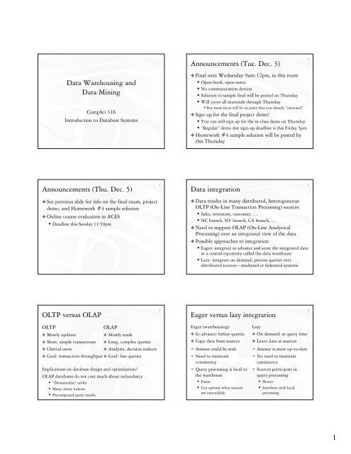
<strong>Announcements</strong> (<strong>Tue</strong>. <strong>Dec</strong>. 3)<br />
2<br />
<strong>Data</strong> <strong>Warehousing</strong> <strong>and</strong><br />
<strong>Data</strong> <strong>Mining</strong><br />
CompSci 316<br />
Introduction to <strong>Data</strong>base Systems<br />
Final next Wednesday 9am-12pm, in this room<br />
Open-book, open-notes<br />
No communication devices<br />
Solution to sample final will be posted on Thursday<br />
Will cover all materials through Thursday<br />
• But more focus will be on parts that you already “exercised”<br />
Sign up for the final project demo!<br />
You can still sign up for the in-class demo on Thursday<br />
“Regular” demo slot sign-up deadline is this Friday 5pm<br />
Homework #4 sample solution will be posted by<br />
this Thursday<br />
<strong>Announcements</strong> (Thu. <strong>Dec</strong>. 5)<br />
3<br />
<strong>Data</strong> integration<br />
4<br />
See previous slide for info on the final exam, project<br />
demo, <strong>and</strong> Homework #4 sample solution<br />
Online course evaluation in ACES<br />
Deadline this Sunday 11:59pm<br />
<strong>Data</strong> resides in many distributed, heterogeneous<br />
OLTP (On-Line Transaction Processing) sources<br />
Sales, inventory, customer, …<br />
NC branch, NY branch, CA branch, …<br />
Need to support OLAP (On-Line Analytical<br />
Processing) over an integrated view of the data<br />
Possible approaches to integration<br />
Eager: integrate in advance <strong>and</strong> store the integrated data<br />
at a central repository called the data warehouse<br />
Lazy: integrate on dem<strong>and</strong>; process queries over<br />
distributed sources—mediated or federated systems<br />
OLTP versus OLAP<br />
5<br />
Eager versus lazy integration<br />
6<br />
OLTP<br />
Mostly updates<br />
OLAP<br />
Mostly reads<br />
Short, simple transactions Long, complex queries<br />
Clerical users<br />
Analysts, decision makers<br />
Goal: transaction throughput Goal: fast queries<br />
Implications on database design <strong>and</strong> optimization?<br />
OLAP databases do not care much about redundancy<br />
“Denormalize” tables<br />
Many, many indexes<br />
Precomputed query results<br />
Eager (warehousing)<br />
In advance: before queries<br />
Copy data from sources<br />
Answer could be stale<br />
Need to maintain<br />
consistency<br />
Query processing is local to<br />
the warehouse<br />
Faster<br />
Can operate when sources<br />
are unavailable<br />
Lazy<br />
On dem<strong>and</strong>: at query time<br />
Leave data at sources<br />
Answer is more up-to-date<br />
No need to maintain<br />
consistency<br />
Sources participate in<br />
query processing<br />
Slower<br />
Interferes with local<br />
processing<br />
1
Maintaining a data warehouse<br />
The “ETL” process<br />
Extraction: extract relevant data <strong>and</strong>/or changes from sources<br />
Transformation: transform data to match the warehouse schema<br />
Loading: integrate data/changes into the warehouse<br />
Approaches<br />
Recomputation<br />
• Easy to implement; just take periodic dumps of the sources, say, every night<br />
• What if there is no “night,” e.g., a global organization?<br />
• What if recomputation takes more than a day?<br />
Incremental maintenance<br />
• Compute <strong>and</strong> apply only incremental changes<br />
• Fast if changes are small<br />
• Not easy to do for complicated transformations<br />
• Need to detect incremental changes at the sources<br />
7<br />
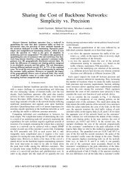
“Star” schema of a data warehouse<br />
Product<br />
Customer<br />
Dimension table<br />
PID name cost<br />
p1 beer 10<br />
p2 diaper 16<br />
… … …<br />
Sale<br />
Dimension table<br />
Store SID city<br />
s1 Durham<br />
OID Date CID PID SID qty price<br />
100 08/23/2012 c3 p1 s1 1 12<br />
Fact table<br />
102 09/12/2012 c3 p2 s1 2 17 Big<br />
105 09/24/2012 c5 p1 s3 5 13<br />
Constantly growing<br />
… … … … … … …<br />
Stores measures (often<br />
aggregated in queries)<br />
CID name address city Dimension table<br />
c3 Amy 100 Main St. Durham Small<br />
c4 Ben 102 Main St. Durham Updated infrequently<br />
c5 Coy 800 Eighth St. Durham<br />
… … … …<br />
s2<br />
s3<br />
…<br />
Chapel Hill<br />
RTP<br />
…<br />
8<br />
<strong>Data</strong> cube<br />
9<br />
Completing the cube—plane<br />
10<br />
Product<br />
p2<br />
p1<br />
Simplified schema: Sale (CID, PID, SID, qty)<br />
(c5, p1, s3) = 5<br />
(c3, p2, s1) = 2<br />
Store<br />
s3<br />
(c3, p1, s1) = 1 (c5, p1, s1) = 3<br />
s2<br />
s1<br />
Total quantity of sales for each product in each store<br />
Product<br />
SELECT PID, SID, SUM(qty) FROM Sale<br />
GROUP BY PID, SID;<br />
(c5, p1, s3) = 5<br />
(ALL, p1, s3) = 5<br />
(ALL, p2, s1) = 2<br />
(c3, p2, s1) = 2<br />
Store<br />
p2 (ALL, p1, s1) = 4 s3<br />
(c3, p1, s1) = 1 (c5, p1, s1) = 3<br />
s2<br />
p1<br />
s1 Project all points onto Product-Store plane<br />
ALL<br />
c3 c4 c5<br />
Customer<br />
ALL<br />
c3 c4 c5<br />
Customer<br />
Completing the cube—axis<br />
11<br />
Completing the cube—origin<br />
12<br />
Product<br />
Total quantity of sales for each product<br />
SELECT PID, SUM(qty) FROM Sale GROUP BY PID;<br />
Product<br />
Total quantity of sales<br />
SELECT SUM(qty) FROM Sale;<br />
(c5, p1, s3) = 5<br />
(ALL, p1, s3) = 5<br />
(ALL, p2, s1) = 2<br />
(c3, p2, s1) = 2<br />
(ALL, p2, ALL)<br />
Store<br />
= 2 p2 (ALL, p1, s1) = 4 s3<br />
(c3, p1, s1) = 1 (c5, p1, s1) = 3<br />
s2<br />
(ALL, p1, ALL)<br />
= 9 p1<br />
s1 Further project points onto Product axis<br />
(c5, p1, s3) = 5<br />
(ALL, p1, s3) = 5<br />
(ALL, p2, s1) = 2<br />
(c3, p2, s1) = 2<br />
(ALL, p2, ALL)<br />
Store<br />
= 2 p2 (ALL, p1, s1) = 4 s3<br />
(c3, p1, s1) = 1 (c5, p1, s1) = 3<br />
s2<br />
(ALL, p1, ALL)<br />
= 9 p1<br />
s1 Further project points onto the origin<br />
ALL<br />
c3 c4 c5<br />
Customer<br />
ALL<br />
(ALL, ALL, ALL) = 11<br />
c3 c4 c5<br />
Customer<br />
2
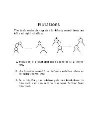
CUBE operator<br />
13<br />
Aggregation lattice<br />
14<br />
Sale (CID, PID, SID, qty)<br />
Proposed SQL extension:<br />
SELECT SUM(qty) FROM Sale<br />
GROUP BY CUBE CID, PID, SID;<br />
Output contains:<br />
Normal groups produced by GROUP BY<br />
• (c1, p1, s1, sum), (c1, p2, s3, sum), etc.<br />
Groups with one or more ALL’s<br />
• (ALL, p1, s1, sum), (c2, ALL, ALL, sum), (ALL, ALL, ALL, sum), etc.<br />
Can you write a CUBE query using only GROUP BY’s?<br />
Gray et al., “<strong>Data</strong> Cube: A Relational Aggregation Operator<br />
Generalizing Group-By, Cross-Tab, <strong>and</strong> Sub-Total.” ICDE 1996<br />
Roll up<br />
Drill down<br />
GROUP BY<br />
CID<br />
GROUP BY<br />
CID, PID<br />
GROUP BY ∅<br />
GROUP BY<br />
PID<br />
GROUP BY<br />
CID, SID<br />
GROUP BY<br />
CID, PID, SID<br />
GROUP BY<br />
SID<br />
GROUP BY<br />
PID, SID<br />
A parent can be<br />
computed from any child<br />
Materialized views<br />
Computing GROUP BY <strong>and</strong> CUBE aggregates is<br />
expensive<br />
OLAP queries perform these operations over <strong>and</strong><br />
over again<br />
Idea: precompute <strong>and</strong> store the aggregates as<br />
materialized views<br />
Maintained automatically as base data changes<br />
No. 1 user-requested feature in PostgreSQL!<br />
15<br />
Selecting views to materialize<br />
Factors in deciding what to materialize<br />
What is its storage cost?<br />
What is its update cost?<br />
Which queries can benefit from it?<br />
How much can a query benefit from it?<br />
Example<br />
GROUP BY ∅ is small, but not useful to most queries<br />
GROUP BY CID, PID, SID is useful to any query, but too large<br />
to be beneficial<br />
Harinarayan et al., “Implementing <strong>Data</strong> Cubes Efficiently.” SIGMOD<br />
1996<br />
16<br />
Other OLAP extensions<br />
Besides extended grouping capabilities (e.g., CUBE),<br />
window operations have also been added to SQL<br />
A “window” specifies an ordered list of rows related<br />
to the “current row”<br />
A window function computes a value from this list<br />
<strong>and</strong> the “current row”<br />
St<strong>and</strong>ard aggregates: COUNT, SUM, AVG, MIN, MAX<br />
New functions: RANK, PERCENT_RANK, LAG, LEAD, …<br />
17<br />
RANK window function example<br />
sid | pid | cid | qty<br />
------------+------------+------------+-----<br />
Durham | beer | Alice | 10<br />
Durham | beer | Bob | 2<br />
Durham | chips | Bob | 3<br />
Durham | diaper | Alice | 5<br />
Raleigh | beer | Alice | 2<br />
Raleigh | diaper | Bob | 100<br />
GROUP BY<br />
sid | pid | cid | qty<br />
------------+------------+------------+-----<br />
Durham | beer | Alice | 10<br />
| | Bob | 2<br />
Durham | chips | Bob | 3<br />
Durham | diaper | Alice | 5<br />
Raleigh | beer | Alice | 2<br />
Raleigh | diaper | Bob | 100<br />
E.g., for the following “row,”<br />
Durham | beer | Alice | 10<br />
| | Bob | 2<br />
SELECT SID, PID, SUM(qty),<br />
RANK() OVER w<br />
FROM Sale GROUP BY SID, PID<br />
WINDOW w AS<br />
(PARTITION BY SID<br />
ORDER BY SUM(qty) DESC);<br />
Apply WINDOW after processing<br />
FROM, WHERE, GROUP BY, HAVING<br />
PARTITION defines the related<br />
set <strong>and</strong> ORDER BY orders it<br />
the related list is:<br />
Durham | beer | Alice | 10<br />
| | Bob | 2<br />
Durham | diaper | Alice | 5<br />
Durham | chips | Bob | 3<br />
18<br />
3
RANK window function example (cont’d) 19<br />
sid | pid | cid | qty<br />
------------+------------+------------+-----<br />
Durham | beer | Alice | 10<br />
| | Bob | 2<br />
Durham | chips | Bob | 3<br />
Durham | diaper | Alice | 5<br />
Raleigh | beer | Alice | 2<br />
Raleigh | diaper | Bob | 100<br />
E.g., for the following “row,”<br />
Durham | beer | Alice | 10<br />
| | Bob | 2<br />
Then, for each “row” <strong>and</strong> its related<br />
list, evaluate SELECT <strong>and</strong> return:<br />
SELECT SID, PID, SUM(qty),<br />
RANK() OVER w<br />
FROM Sale GROUP BY SID, PID<br />
WINDOW w AS<br />
(PARTITION BY SID<br />
ORDER BY SUM(qty) DESC);<br />
the related list is:<br />
sid | pid | sum | rank<br />
------------+------------+-----+------<br />
Durham | beer | 12 | 1<br />
Durham | diaper | 5 | 2<br />
Durham | chips | 3 | 3<br />
Raleigh | diaper | 100 | 1<br />
Raleigh | beer | 2 | 2<br />
Durham | beer | Alice | 10<br />
| | Bob | 2<br />
Durham | diaper | Alice | 5<br />
Durham | chips | Bob | 3<br />
Multiple windows<br />
sid | pid | cid | qty<br />
------------+------------+------------+-----<br />
Durham | beer | Alice | 10<br />
| | Bob | 2<br />
Durham | chips | Bob | 3<br />
Durham | diaper | Alice | 5<br />
Raleigh | beer | Alice | 2<br />
Raleigh | diaper | Bob | 100<br />
No PARTITION means all “rows”<br />
are related to the current one<br />
So rank1 is the “global” rank:<br />
SELECT SID, PID, SUM(qty),<br />
RANK() OVER w,<br />
RANK() OVER w1 AS rank1<br />
FROM Sale GROUP BY SID, PID<br />
WINDOW w AS<br />
(PARTITION BY SID<br />
ORDER BY SUM(qty) DESC),<br />
w1 AS<br />
(ORDER BY SUM(qty) DESC)<br />
ORDER BY SID, rank;<br />
sid | pid | sum | rank | rank1<br />
------------+------------+-----+------+-------<br />
Durham | beer | 12 | 1 | 2<br />
Durham | diaper | 5 | 2 | 3<br />
Durham | chips | 3 | 3 | 4<br />
Raleigh | diaper | 100 | 1 | 1<br />
Raleigh | beer | 2 | 2 | 5<br />
20<br />
<strong>Data</strong> mining<br />
21<br />
<strong>Mining</strong> frequent itemsets<br />
22<br />
<strong>Data</strong> → knowledge<br />
DBMS meets AI <strong>and</strong> statistics<br />
Clustering, prediction (classification <strong>and</strong> regression),<br />
association analysis, outlier analysis, evolution<br />
analysis, etc.<br />
Usually complex statistical “queries” that are difficult to<br />
answer → often specialized algorithms outside DBMS<br />
We will focus on frequent itemset mining<br />
Given: a large database of<br />
transactions, each containing<br />
a set of items<br />
Example: market baskets<br />
Find all frequent itemsets<br />
A set of items is frequent if<br />
no less than % of all<br />
transactions contain X<br />
Examples: {diaper, beer},<br />
{scanner, color printer}<br />
TID<br />
T001<br />
T002<br />
T003<br />
T004<br />
T005<br />
T006<br />
T007<br />
T008<br />
T009<br />
…<br />
items<br />
diaper, milk, c<strong>and</strong>y<br />
milk, egg<br />
milk, beer<br />
diaper, milk, egg<br />
diaper, beer<br />
milk, beer<br />
diaper, beer<br />
diaper, milk, beer, c<strong>and</strong>y<br />
diaper, milk, beer<br />
…<br />
First try<br />
23<br />
The Apriori property<br />
24<br />
A naïve algorithm<br />
Keep a running count for each possible itemset<br />
For each transaction , <strong>and</strong> for each itemset , if <br />
contains then increment the count for <br />
Return itemsets with large enough counts<br />
Problem: The number of itemsets is huge!<br />
2 , where is the number of items<br />
Think: How do we prune the search space?<br />
All subsets of a frequent itemset must also be<br />
frequent<br />
Because any transaction that contains must also<br />
contains subsets of <br />
If we have already verified that is infrequent,<br />
there is no need to count ’s supersets because they<br />
must be infrequent too<br />
4
The Apriori algorithm<br />
Multiple passes over the transactions<br />
Pass finds all frequent -itemsets (i.e., itemsets of<br />
size )<br />
Use the set of frequent -itemsets found in pass to<br />
construct c<strong>and</strong>idate + 1 -itemsets to be counted<br />
in pass + 1<br />
A + 1 -itemset is a c<strong>and</strong>idate only if all its subsets of<br />
size are frequent<br />
25<br />
Example: pass 1<br />
TID items<br />
T001 A, B, E<br />
T002 B, D<br />
T003 B, C<br />
T004 A, B, D<br />
T005 A, C<br />
itemset count<br />
T006 B, C<br />
{A} 6<br />
T007 A, C<br />
{B} 7<br />
T008 A, B, C, E<br />
{C} 6<br />
T009 A, B, C<br />
{D} 2<br />
T010 F<br />
{E} 2<br />
Transactions<br />
% = 20%<br />
Frequent 1-itemsets<br />
(Itemset {F} is infrequent)<br />
26<br />
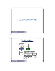
Example: pass 2<br />
TID<br />
T001<br />
T002<br />
T003<br />
T004<br />
T005<br />
T006<br />
T007<br />
T008<br />
T009<br />
T010<br />
items<br />
A, B, E<br />
B, D<br />
B, C<br />
A, B, D<br />
A, C<br />
B, C<br />
A, C<br />
A, B, C, E<br />
A, B, C<br />
F<br />
Transactions<br />
% = 20%<br />
itemset<br />
{A} 6<br />
{B} 7<br />
{C} 6<br />
{D} 2<br />
{E} 2<br />
Frequent<br />
1-itemsets<br />
Generate<br />
c<strong>and</strong>idates<br />
count<br />
Scan <strong>and</strong><br />
count<br />
itemset<br />
{A,B} 4<br />
{A,C} 4<br />
{A,D} 1<br />
{A,E} 2<br />
{B,C} 4<br />
{B,D} 2<br />
{B,E} 2<br />
{C,D} 0<br />
{C,E} 1<br />
count<br />
{D,E} 0<br />
C<strong>and</strong>idate<br />
2-itemsets<br />
Check<br />
min. support<br />
itemset<br />
{A,B} 4<br />
{A,C} 4<br />
{A,E} 2<br />
{B,C} 4<br />
{B,D} 2<br />
{B,E} 2<br />
count<br />
Frequent<br />
2-itemsets<br />
27<br />
Example: pass 3<br />
TID<br />
T001<br />
T002<br />
T003<br />
T004<br />
T005<br />
T006<br />
T007<br />
T008<br />
T009<br />
T010<br />
items<br />
A, B, E<br />
B, D<br />
B, C<br />
A, B, D<br />
A, C<br />
B, C<br />
A, C<br />
A, B, C, E<br />
A, B, C<br />
F<br />
Transactions<br />
% = 20%<br />
itemset<br />
{A,B} 4<br />
{A,C} 4<br />
{A,E} 2<br />
{B,C} 4<br />
{B,D} 2<br />
{B,E} 2<br />
Frequent<br />
2-itemsets<br />
Generate<br />
c<strong>and</strong>idates<br />
count<br />
Scan <strong>and</strong><br />
count<br />
itemset<br />
{A,B,C} 2<br />
{A,B,E} 2<br />
count<br />
C<strong>and</strong>idate<br />
3-itemsets<br />
Check<br />
min. support<br />
itemset<br />
{A,B,C} 2<br />
count<br />
{A,B,E} 2<br />
Frequent<br />
3-itemsets<br />
28<br />
Example: pass 4<br />
29<br />
Example: final answer<br />
30<br />
TID<br />
T001<br />
T002<br />
T003<br />
T004<br />
T005<br />
T006<br />
T007<br />
T008<br />
T009<br />
T010<br />
items<br />
A, B, E<br />
B, D<br />
B, C<br />
A, B, D<br />
A, C<br />
B, C<br />
A, C<br />
A, B, C, E<br />
A, B, C<br />
F<br />
Transactions<br />
% = 20%<br />
itemset<br />
{A,B,C} 2<br />
{A,B,E} 2<br />
Frequent<br />
3-itemsets<br />
Generate<br />
c<strong>and</strong>idates<br />
count<br />
itemset<br />
count<br />
C<strong>and</strong>idate<br />
4-itemsets<br />
No more itemsets to count!<br />
itemset<br />
{A} 6<br />
{B} 7<br />
{C} 6<br />
{D} 2<br />
{E} 2<br />
count<br />
Frequent<br />
1-itemsets<br />
itemset<br />
{A,B} 4<br />
{A,C} 4<br />
{A,E} 2<br />
{B,C} 4<br />
{B,D} 2<br />
{B,E} 2<br />
count<br />
Frequent<br />
2-itemsets<br />
itemset<br />
{A,B,C} 2<br />
{A,B,E} 2<br />
count<br />
Frequent<br />
3-itemsets<br />
5
Summary<br />
<strong>Data</strong> warehousing<br />
Eagerly integrate data from operational sources <strong>and</strong> store<br />
a redundant copy to support OLAP<br />
OLAP vs. OLTP: different workload → different degree<br />
of redundancy<br />
SQL extensions: grouping <strong>and</strong> windowing<br />
<strong>Data</strong> mining<br />
Only covered frequent itemset counting<br />
Skipped many other techniques (clustering, classification,<br />
regression, etc.)<br />
One key difference from statistics <strong>and</strong> machine learning:<br />
massive datasets <strong>and</strong> I/O-efficient algorithms<br />
31<br />
6