FORWARD KINEMATICS: THE DENAVIT-HARTENBERG ...

Chapter 3
FORWARD KINEMATICS:
THE
DENAVIT-HARTENBERG
CONVENTION
In this chapter we develop the forward or configuration kinematic equations
for rigid robots. The forward kinematics problem is concerned with
the relationship between the individual joints of the robot manipulator and
the position and orientation of the tool or end-effector. Stated more formally,
the forward kinematics problem is to determine the position and orientation
of the end-effector, given the values for the joint variables of the robot. The
joint variables are the angles between the links in the case of revolute or
rotational joints, and the link extension in the case of prismatic or sliding
joints. The forward kinematics problem is to be contrasted with the inverse
kinematics problem, which will be studied in the next chapter, and which
is concerned with determining values for the joint variables that achieve a
desired position and orientation for the end-effector of the robot.
3.1 Kinematic Chains
As described in Chapter 1, a robot manipulator is composed of a set of
links connected together by various joints. The joints can either be very
simple, such as a revolute joint or a prismatic joint, or else they can be more
complex, such as a ball and socket joint. (Recall that a revolute joint is like
71

72CHAPTER 3. FORWARD KINEMATICS: THE DENAVIT-HARTENBERG CONVENTION
a hinge and allows a relative rotation about a single axis, and a prismatic
joint permits a linear motion along a single axis, namely an extension or
retraction.) The difference between the two situations is that, in the first
instance, the joint has only a single degree-of-freedom of motion: the angle of
rotation in the case of a revolute joint, and the amount of linear displacement
in the case of a prismatic joint. In contrast, a ball and socket joint has two
degrees-of-freedom. In this book it is assumed throughout that all joints
have only a single degree-of-freedom. Note that the assumption does not
involve any real loss of generality, since joints such as a ball and socket joint
(two degrees-of-freedom) or a spherical wrist (three degrees-of-freedom) can
always be thought of as a succession of single degree-of-freedom joints with
links of length zero in between.
With the assumption that each joint has a single degree-of-freedom, the
action of each joint can be described by a single real number: the angle of
rotation in the case of a revolute joint or the displacement in the case of a
prismatic joint. The objective of forward kinematic analysis is to determine
the cumulative effect of the entire set of joint variables. In this chapter
we will develop a set of conventions that provide a systematic procedure
for performing this analysis. It is, of course, possible to carry out forward
kinematics analysis even without respecting these conventions, as we did
for the two-link planar manipulator example in Chapter 1. However, the
kinematic analysis of an n-link manipulator can be extremely complex and
the conventions introduced below simplify the analysis considerably. Moreover,
they give rise to a universal language with which robot engineers can
communicate.
A robot manipulator with n joints will have n + 1 links, since each joint
connects two links. We number the joints from 1 to n, and we number the
links from 0 to n, starting from the base. By this convention, joint i connects
link i − 1 to link i. We will consider the location of joint i to be fixed with
respect to link i − 1. When joint i is actuated, link i moves. Therefore, link
0 (the first link) is fixed, and does not move when the joints are actuated.
Of course the robot manipulator could itself be mobile (e.g., it could be
mounted on a mobile platform or on an autonomous vehicle), but we will
not consider this case in the present chapter, since it can be handled easily
by slightly extending the techniques presented here.
With the i th joint, we associate a joint variable, denoted by qi. In the
case of a revolute joint, qi is the angle of rotation, and in the case of a

3.1. KINEMATIC CHAINS 73
z1
x0
y1
z0
θ2
θ1
z2
θ3
x1 x2 x3
y0
y2
Figure 3.1: Coordinate frames attached to elbow manipulator.
prismatic joint, qi is the joint displacement:
�
qi =
z3
y3
θi : joint i revolute
di : joint i prismatic
. (3.1)
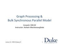
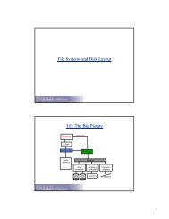
To perform the kinematic analysis, we rigidly attach a coordinate frame
to each link. In particular, we attach oixiyizi to link i. This means that,
whatever motion the robot executes, the coordinates of each point on link
i are constant when expressed in the i th coordinate frame. Furthermore,
when joint i is actuated, link i and its attached frame, oixiyizi, experience
a resulting motion. The frame o0x0y0z0, which is attached to the robot
base, is referred to as the inertial frame. Figure 3.1 illustrates the idea of
attaching frames rigidly to links in the case of an elbow manipulator.
Now suppose Ai is the homogeneous transformation matrix that expresses
the position and orientation of oixiyizi with respect to oi−1xi−1yi−1zi−1.
The matrix Ai is not constant, but varies as the configuration of the robot
is changed. However, the assumption that all joints are either revolute or
prismatic means that Ai is a function of only a single joint variable, namely
qi. In other words,
Ai = Ai(qi). (3.2)
Now the homogeneous transformation matrix that expresses the position
and orientation of ojxjyjzj with respect to oixiyizi is called, by convention,
a transformation matrix, and is denoted by T i
j. From Chapter 2 we see
that
T i
j = Ai+1Ai+2 ...Aj−1Aj if i < j

74CHAPTER 3. FORWARD KINEMATICS: THE DENAVIT-HARTENBERG CONVENTION
T i
j = I if i = j (3.3)
T i
j = (T j
i ) −1 if j > i.
By the manner in which we have rigidly attached the various frames
to the corresponding links, it follows that the position of any point on the
end-effector, when expressed in frame n, is a constant independent of the
configuration of the robot. Denote the position and orientation of the end-
effector with respect to the inertial or base frame by a three-vector O 0
n
(which gives the coordinates of the origin of the end-effector frame with
respect to the base frame) and the 3 × 3 rotation matrix R 0
n, and define the
homogeneous transformation matrix
�
H =
R 0
n O 0
n
0 1
�
. (3.4)
Then the position and orientation of the end-effector in the inertial frame
are given by
H = T 0
n = A1(q1) · · ·An(qn). (3.5)
Each homogeneous transformation Ai is of the form
�
R
Ai =
i−1
i O i−1
�
i . (3.6)
0 1
Hence
T i
j = Ai+1 · · ·Aj =
�
R i
j O i
j
0 1
�
. (3.7)
The matrix R i
j expresses the orientation of ojxjyjzj relative to oixiyizi
and is given by the rotational parts of the A-matrices as
The coordinate vectors O i
j
R i
j = R i
i+1 · · ·R j−1
j . (3.8)
are given recursively by the formula
O i
j = O i
j−1 + R i
j−1O j−1
j , (3.9)
These expressions will be useful in Chapter 5 when we study Jacobian matrices.
In principle, that is all there is to forward kinematics! Determine the
functions Ai(qi), and multiply them together as needed. However, it is possible
to achieve a considerable amount of streamlining and simplification by
introducing further conventions, such as the Denavit-Hartenberg representation
of a joint, and this is the objective of the remainder of the chapter.

3.2. DENAVIT HARTENBERG REPRESENTATION 75
3.2 Denavit Hartenberg Representation
While it is possible to carry out all of the analysis in this chapter using an
arbitrary frame attached to each link, it is helpful to be systematic in the
choice of these frames. A commonly used convention for selecting frames of
reference in robotic applications is the Denavit-Hartenberg, or D-H convention.
In this convention, each homogeneous transformation Ai is represented
as a product of four basic transformations
Ai = R z,θi Transz,di Transx,ai R x,α i
=
=
⎡
⎢
⎣
⎡
⎢
⎣
cθi −sθi 0 0
sθi cθi 0 0
0 0 1 0
0 0 0 1
⎤ ⎡
⎥ ⎢
⎥ ⎢
⎥ ⎢
⎦ ⎣
1 0 0 0
0 1 0 0
0 0 1 di
0 0 0 1
⎤
cθi −sθi cαi sθi sαi aicθi
sθi
cθicαi −cθisαi aisθi
0 sαi
cαi di
0 0 0 1
⎥
⎦
⎤ ⎡
⎥ ⎢
⎥ ⎢
⎥ ⎢
⎦ ⎣
1 0 0 ai
0 1 0 0
0 0 1 0
0 0 0 1
(3.10)
⎤ ⎡
1 0
⎥ ⎢
⎥ ⎢ 0 cαi
⎥ ⎢
⎦ ⎣
0 0
−sαi
0 sαi
0 0
cαi
0
⎤
0
⎥
0 ⎦
1
where the four quantities θi, ai, di, αi are parameters associated with link
i and joint i. The four parameters ai,αi,di, and θi in (3.10) are generally
given the names link length, link twist, link offset, and joint angle,
respectively. These names derive from specific aspects of the geometric
relationship between two coordinate frames, as will become apparent below.
Since the matrix Ai is a function of a single variable, it turns out that three
of the above four quantities are constant for a given link, while the fourth
parameter, θi for a revolute joint and di for a prismatic joint, is the joint
variable.
From Chapter 2 one can see that an arbitrary homogeneous transformation
matrix can be characterized by six numbers, such as, for example, three
numbers to specify the fourth column of the matrix and three Euler angles
to specify the upper left 3×3 rotation matrix. In the D-H representation, in
contrast, there are only four parameters. How is this possible? The answer
is that, while frame i is required to be rigidly attached to link i, we have
considerable freedom in choosing the origin and the coordinate axes of the
frame. For example, it is not necessary that the origin, O i , of frame i be
placed at the physical end of link i. In fact, it is not even necessary that
frame i be placed within the physical link; frame i could lie in free space —
so long as frame i is rigidly attached to link i. By a clever choice of the origin
and the coordinate axes, it is possible to cut down the number of parameters

76CHAPTER 3. FORWARD KINEMATICS: THE DENAVIT-HARTENBERG CONVENTION
d
θ
y0
x0
z0
O0
Figure 3.2: Coordinate frames satisfying assumptions DH1 and DH2.
needed from six to four (or even fewer in some cases). In Section 3.2.1 we
will show why, and under what conditions, this can be done, and in Section
3.2.2 we will show exactly how to make the coordinate frame assignments.
3.2.1 Existence and uniqueness issues
Clearly it is not possible to represent any arbitrary homogeneous transformation
using only four parameters. Therefore, we begin by determining just
which homogeneous transformations can be expressed in the form (3.10).
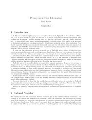
Suppose we are given two frames, denoted by frames 0 and 1, respectively.
Then there exists a unique homogeneous transformation matrix A that takes
the coordinates from frame 1 into those of frame 0. Now suppose the two
frames have two additional features, namely:
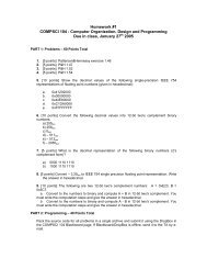
(DH1) The axis x1 is perpendicular to the axis z0
(DH2) The axis x1 intersects the axis z0
as shown in Figure 3.2. Under these conditions, we claim that there exist
unique numbers a, d, θ, α such that
a
x1
α
z1
O1
A = R z,θTransz,dTransx,aR x,α. (3.11)
Of course, since θ and α are angles, we really mean that they are unique to
within a multiple of 2π. To show that the matrix A can be written in this
y1

3.2. DENAVIT HARTENBERG REPRESENTATION 77
form, write A as
A =
�
R 0
1 O 0
1
0 1
�
(3.12)
and let ri denote the i th column of the rotation matrix R 0
1. We will now
examine the implications of the two DH constraints.
If (DH1) is satisfied, then x1 is perpendicular to z0 and we have x1·z0 = 0.
Expressing this constraint with respect to o0x0y0z0, using the fact that r1 is
the representation of the unit vector x1 with respect to frame 0, we obtain
0 = x 0
1 · z 0
0
= [r11,r21,r31] T · [0,0, 1] T
(3.13)
(3.14)
= r31. (3.15)
Since r31 = 0, we now need only show that there exist unique angles θ and
α such that
⎡
⎤
R 0
1 = R x,θR x,α =
⎢
⎣
cθ −sθcα sθsα
sθ cθcα −cθsα
0 sα cα
⎥
⎦. (3.16)
The only information we have is that r31 = 0, but this is enough. First,
since each row and column of R 0
1 must have unit length, r31 = 0 implies that
r 2 11 + r 2 21 = 1,
Hence there exist unique θ, α such that
r 2 32 + r 2 33 = 1 (3.17)
(r11,r21) = (cθ,sθ), (r33,r32) = (cα,sα). (3.18)
Once θ and α are found, it is routine to show that the remaining elements of
R 0
1 must have the form shown in (3.16), using the fact that R 0
1 is a rotation
matrix.
Next, assumption (DH2) means that the displacement between O 0 and
O 1 can be expressed as a linear combination of the vectors z0 and x1. This
can be written as O 1 = O 0 +dz0 +ax1. Again, we can express this relationship
in the coordinates of o0x0y0z0, and we obtain
O 0
1 = O 0
0 + dz 0
0 + ax 0
1
(3.19)

78CHAPTER 3. FORWARD KINEMATICS: THE DENAVIT-HARTENBERG CONVENTION
=
=
⎡
⎢
⎣
⎡
⎢
⎣
0
0
0
⎤
acθ
asθ
d
⎡
⎥ ⎢
⎦ + d ⎣
⎤
⎤ ⎡ ⎤
cθ
⎥ ⎢ ⎥
⎦ + a ⎣ ⎦ (3.20)
0
0
1
sθ
0
⎥
⎦. (3.21)
Combining the above results, we obtain (3.10) as claimed. Thus, we see
that four parameters are sufficient to specify any homogeneous transformation
that satisfies the constraints (DH1) and (DH2).
Now that we have established that each homogeneous transformation
matrix satisfying conditions (DH1) and (DH2) above can be represented
in the form (3.10), we can in fact give a physical interpretation to each
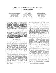
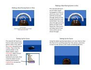
of the four quantities in (3.10). The parameter a is the distance between
the axes z0 and z1, and is measured along the axis x1. The angle α is the
angle between the axes z0 and z1, measured in a plane normal to x1. The
positive sense for α is determined from z0 to z1 by the right-hand rule as
shown in Figure 3.3. The parameter d is the distance between the origin
xi
zi
αi zi−1
xi−1
xi
Figure 3.3: Positive sense for αi and θi.
zi−1
O 0 and the intersection of the x1 axis with z0 measured along the z0 axis.
Finally, θ is the angle between x0 and x1 measured in a plane normal to z0.
These physical interpretations will prove useful in developing a procedure for
assigning coordinate frames that satisfy the constraints (DH1) and (DH2),
and we now turn our attention to developing such a procedure.
θi

3.2. DENAVIT HARTENBERG REPRESENTATION 79
3.2.2 Assigning the coordinate frames
For a given robot manipulator, one can always choose the frames 0,...,n in
such a way that the above two conditions are satisfied. In certain circumstances,
this will require placing the origin Oi of frame i in a location that
may not be intuitively satisfying, but typically this will not be the case. In
reading the material below, it is important to keep in mind that the choices
of the various coordinate frames are not unique, even when constrained by
the requirements above. Thus, it is possible that different engineers will
derive differing, but equally correct, coordinate frame assignments for the
links of the robot. It is very important to note, however, that the end result
(i.e., the matrix T 0
n) will be the same, regardless of the assignment of
intermediate link frames (assuming that the coordinate frames for link n
coincide). We will begin by deriving the general procedure. We will then
discuss various common special cases where it is possible to further simplify
the homogeneous transformation matrix.
To start, note that the choice of zi is arbitrary. In particular, from (3.16),
we see that by choosing αi and θi appropriately, we can obtain any arbitrary
direction for zi. Thus, for our first step, we assign the axes z0,...,zn−1 in
an intuitively pleasing fashion. Specifically, we assign zi to be the axis of
actuation for joint i + 1. Thus, z0 is the axis of actuation for joint 1, z1 is
the axis of actuation for joint 2, etc. There are two cases to consider: (i) if
joint i + 1 is revolute, zi is the axis of revolution of joint i + 1; (ii) if joint
i + 1 is prismatic, zi is the axis of translation of joint i + 1. At first it may
seem a bit confusing to associate zi with joint i + 1, but recall that this
satisfies the convention that we established in Section 3.1, namely that joint
i is fixed with respect to frame i, and that when joint i is actuated, link i
and its attached frame, oixiyizi, experience a resulting motion.
Once we have established the z-axes for the links, we establish the base
frame. The choice of a base frame is nearly arbitrary. We may choose the
origin O0 of the base frame to be any point on z0. We then choose x0, y0 in
any convenient manner so long as the resulting frame is right-handed. This
sets up frame 0.
Once frame 0 has been established, we begin an iterative process in which
we define frame i using frame i − 1, beginning with frame 1. Figure 3.4 will
be useful for understanding the process that we now describe.
In order to set up frame i it is necessary to consider three cases: (i) the
axes zi−1, zi are not coplanar, (ii) the axes zi−1, zi intersect (iii) the axes
zi−1, zi are parallel. Note that in both cases (ii) and (iii) the axes zi−1 and
zi are coplanar. This situation is in fact quite common, as we will see in

80CHAPTER 3. FORWARD KINEMATICS: THE DENAVIT-HARTENBERG CONVENTION
Figure 3.4: Denavit-Hartenberg frame assignment.
Section 3.3. We now consider each of these three cases.
(i) zi−1 and zi are not coplanar: If zi−l and zi are not coplanar, then
there exists a unique line segment perpendicular to both zi−1 and zi such
that it connects both lines and it has minimum length. The line containing
this common normal to zi−1 and zi defines xi, and the point where this line
intersects zi is the origin O i . By construction, both conditions (DH1) and
(DH2) are satisfied and the vector from O i−1 to O i is a linear combination
of zi−1 and xi. The specification of frame i is completed by choosing the
axis yi to form a right-hand frame. Since assumptions (DH1) and (DH2) are
satisfied the homogeneous transformation matrix Ai is of the form (3.10).
(ii) zi−1 is parallel to zi: If the axes zi−1 and zi are parallel, then there are
infinitely many common normals between them and condition (DH1) does
not specify xi completely. In this case we are free to choose the origin O i
anywhere along zi. One often chooses O i to simplify the resulting equations.
The axis xi is then chosen either to be directed from O i toward zi−1, along
the common normal, or as the opposite of this vector. A common method
for choosing O i is to choose the normal that passes through O i−1 as the xi
axis; O i is then the point at which this normal intersects zi. In this case, di
would be equal to zero. Once xi is fixed, yi is determined, as usual by the
right hand rule. Since the axes zi−1 and zi are parallel, αi will be zero in
this case.
(iii) zi−1 intersects zi: In this case xi is chosen normal to the plane
formed by zi and zi−1. The positive direction of xi is arbitrary. The most

3.2. DENAVIT HARTENBERG REPRESENTATION 81
natural choice for the origin O i in this case is at the point of intersection of
zi and zi−1. However, any convenient point along the axis zi suffices. Note
that in this case the parameter ai equals 0.
This constructive procedure works for frames 0,...,n − l in an n-link
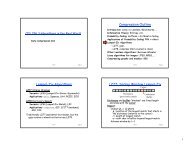
robot. To complete the construction, it is necessary to specify frame n.
The final coordinate system onxnynzn is commonly referred to as the endeffector
or tool frame (see Figure 3.5). The origin O n is most often
O0
x0
z0
Note: currently rendering
a 3D gripper...
y0
On
xn ≡ n
Figure 3.5: Tool frame assignment.
yn ≡ s
zn ≡ a
placed symmetrically between the fingers of the gripper. The unit vectors
along the xn, yn, and zn axes are labeled as n, s, and a, respectively. The
terminology arises from fact that the direction a is the approach direction,
in the sense that the gripper typically approaches an object along the a
direction. Similarly the s direction is the sliding direction, the direction
along which the fingers of the gripper slide to open and close, and n is the
direction normal to the plane formed by a and s.
In contemporary robots the final joint motion is a rotation of the endeffector
by θn and the final two joint axes, zn−1 and zn, coincide. In this
case, the transformation between the final two coordinate frames is a translation
along zn−1 by a distance dn followed (or preceded) by a rotation of
θn radians about zn−1. This is an important observation that will simplify
the computation of the inverse kinematics in the next chapter.
Finally, note the following important fact. In all cases, whether the joint
in question is revolute or prismatic, the quantities ai and αi are always
constant for all i and are characteristic of the manipulator. If joint i is prismatic,
then θi is also a constant, while di is the i th joint variable. Similarly,
if joint i is revolute, then di is constant and θi is the i th joint variable.

82CHAPTER 3. FORWARD KINEMATICS: THE DENAVIT-HARTENBERG CONVENTION
3.2.3 Summary
We may summarize the above procedure based on the D-H convention in the
following algorithm for deriving the forward kinematics for any manipulator.
Step l: Locate and label the joint axes z0,...,zn−1.
Step 2: Establish the base frame. Set the origin anywhere on the z0-axis.
The x0 and y0 axes are chosen conveniently to form a right-hand frame.
For i = 1,...,n − 1, perform Steps 3 to 5.
Step 3: Locate the origin O i where the common normal to zi and zi−1
intersects zi. If zi intersects zi−1 locate O i at this intersection. If zi
and zi−1 are parallel, locate O i in any convenient position along zi.
Step 4: Establish xi along the common normal between zi−1 and zi through
O i , or in the direction normal to the zi−1 − zi plane if zi−1 and zi
intersect.
Step 5: Establish yi to complete a right-hand frame.
Step 6: Establish the end-effector frame onxnynzn. Assuming the n-th joint
is revolute, set zn = a along the direction zn−1. Establish the origin
O n conveniently along zn, preferably at the center of the gripper or at
the tip of any tool that the manipulator may be carrying. Set yn = s
in the direction of the gripper closure and set xn = n as s × a. If
the tool is not a simple gripper set xn and yn conveniently to form a
right-hand frame.
Step 7: Create a table of link parameters ai, di, αi, θi.
ai = distance along xi from O i to the intersection of the xi and zi−1
axes.
di = distance along zi−1 from O i−1 to the intersection of the xi and
zi−1 axes. di is variable if joint i is prismatic.
αi = the angle between zi−1 and zi measured about xi (see Figure
3.3).
θi = the angle between xi−1 and xi measured about zi−1 (see Figure
3.3). θi is variable if joint i is revolute.
Step 8: Form the homogeneous transformation matrices Ai by substituting
the above parameters into (3.10).

3.3. EXAMPLES 83
Step 9: Form T 0
n = A1 · · ·An. This then gives the position and orientation
of the tool frame expressed in base coordinates.
3.3 Examples
In the D-H convention the only variable angle is θ, so we simplify notation
by writing ci for cos θi, etc. We also denote θ1 + θ2 by θ12, and cos(θ1 + θ2)
by c12, and so on. In the following examples it is important to remember
that the D-H convention, while systematic, still allows considerable freedom
in the choice of some of the manipulator parameters. This is particularly
true in the case of parallel joint axes or when prismatic joints are involved.
Example 3.1 Planar Elbow Manipulator
Consider the two-link planar arm of Figure 3.6. The joint axes z0 and
y0
a1
y1
θ1
y2
a2
Figure 3.6: Two-link planar manipulator. The z-axes all point out of the
page, and are not shown in the figure.
z1 are normal to the page. We establish the base frame o0x0y0z0 as shown.
The origin is chosen at the point of intersection of the z0 axis with the page
and the direction of the x0 axis is completely arbitrary. Once the base frame
is established, the o1x1y1z1 frame is fixed as shown by the D-H convention,
where the origin O 1 has been located at the intersection of z1 and the page.
The final frame o2x2y2z2 is fixed by choosing the origin O 2 at the end of link 2
as shown. The link parameters are shown in Table 3.1. The A-matrices are
θ2
x0
x2
x1

84CHAPTER 3. FORWARD KINEMATICS: THE DENAVIT-HARTENBERG CONVENTION
Table 3.1: Link parameters for 2-link planar manipulator.
determined from (3.10) as
The T-matrices are thus given by
Link ai αi di θi
1 a1 0 0 θ ∗ 1
2 a2 0 0 θ ∗ 2
∗ variable
A1 =
⎡
c1
⎢ s1
⎢
⎣ 0
−s1
c1
0
⎤
0 a1c1
0
⎥
a1s1 ⎥
⎥.
1 0 ⎦
(3.22)
A2 =
0
⎡
c2
⎢ s2
⎢
⎣ 0
0
−s2
c2
0
0 1
⎤
0 a2c2
0
⎥
a2s2 ⎥
1 0 ⎦
(3.23)
0 0 0 1
T 0
1 = A1. (3.24)
⎡
⎤
T 0
2
c12
⎢ s12
= A1A2 = ⎢
⎣ 0
−s12
c12
0
0 a1c1 + a2c12
0 a1s1 + a2s12
1 0
0 0 0 1
⎥
⎥.
(3.25)
⎦
Notice that the first two entries of the last column of T 0
2 are the x and y
components of the origin O 2 in the base frame; that is,
x = a1c1 + a2c12
y = a1s1 + a2s12
(3.26)
are the coordinates of the end-effector in the base frame. The rotational part
of T 0
2 gives the orientation of the frame o2x2y2z2 relative to the base frame.
⋄
Example 3.2 Three-Link Cylindrical Robot
Consider now the three-link cylindrical robot represented symbolically by
Figure 3.7. We establish O 0 as shown at joint 1. Note that the placement of

3.3. EXAMPLES 85
x2
d2
x1
x0
d3
O2
y2
z1
O1
θ1
z0
O0
z2
y1
y0
x3
O3
Figure 3.7: Three-link cylindrical manipulator.
Table 3.2: Link parameters for 3-link cylindrical manipulator.
y3
Link ai αi di θi
1 0 0 d1 θ ∗ 1
2 0 −90 d ∗ 2 0
3 0 0 d ∗ 3 0
∗ variable
the origin O 0 along z0 as well as the direction of the x0 axis are arbitrary.
Our choice of O 0 is the most natural, but O 0 could just as well be placed
at joint 2. The axis x0 is chosen normal to the page. Next, since z0 and
z1 coincide, the origin O 1 is chosen at joint 1 as shown. The x1 axis is
normal to the page when θ1 = 0 but, of course its direction will change since
θ1 is variable. Since z2 and z1 intersect, the origin O 2 is placed at this
intersection. The direction of x2 is chosen parallel to x1 so that θ2 is zero.
Finally, the third frame is chosen at the end of link 3 as shown.
The link parameters are now shown in Table 3.2. The corresponding A
z3

86CHAPTER 3. FORWARD KINEMATICS: THE DENAVIT-HARTENBERG CONVENTION
and T matrices are
⋄
A1 =
A2 =
A3 =
T 0
3 = A1A2A3 =
⎡
⎢
⎣
⎡
⎢
⎣
⎡
⎢
⎣
Example 3.3 Spherical Wrist
x4
z4
z3,
x5
z5
θ4
θ5
c1 −s1 0 0
s1 c1 0 0
0 0 1 d1
0 0 0 1
1 0 0 0
0 0 1 0
0 −1 0 d2
0 0 0 1
1 0 0 0
0 1 0 0
0 0 1 d3
0 0 0 1
⎤
⎥
⎦
⎤
⎥
⎦
⎤
⎥
⎦
(3.27)
⎡
c1
⎢ s1
⎢
⎣ 0
0
0
−1
−s1
c1
0
⎤
−s1d3
⎥
c1d3 ⎥
⎥.
d1 + d2 ⎦
(3.28)
0 0 0 1
θ6
To gripper
Figure 3.8: The spherical wrist frame assignment.
The spherical wrist configuration is shown in Figure 3.8, in which the
joint axes z3, z4, z5 intersect at O. The Denavit-Hartenberg parameters are
shown in Table 3.3. The Stanford manipulator is an example of a manipulator
that possesses a wrist of this type. In fact, the following analysis applies
to virtually all spherical wrists.

3.3. EXAMPLES 87
Table 3.3: DH parameters for spherical wrist.
Link ai αi di θi
4 0 −90 0 θ ∗ 4
5 0 90 0 θ ∗ 5
6 0 0 d6 θ ∗ 6
∗ variable
We show now that the final three joint variables, θ4, θ5, θ6 are the Euler
angles φ, θ, ψ, respectively, with respect to the coordinate frame o3x3y3z3. To
see this we need only compute the matrices A4, A5, and A6 using Table 3.3
and the expression (3.10). This gives
T 3
6 = A4A5A6 =
A4 =
A5 =
A6 =
⎡
⎢
⎣
⎡
⎢
⎣
⎡
⎢
⎣
Multiplying these together yields
� �
=
R 3
6 O 3
6
0 1
c4 0 −s4 0
s4 0 c4 0
0 −1 0 0
0 0 0 1
c5 0 s5 0
s5 0 −c5 0
0 −1 0 0
0 0 0 1
c6 −s6 0 0
s6 c6 0 0
0 0 1 d6
0 0 0 1
⎤
⎥
⎦
⎤
⎥
⎦
⎤
(3.29)
(3.30)
⎥
⎥.
(3.31)
⎦
⎡
c4c5c6 − s4s6
⎢ s4c5c6 + c4s6
⎢
⎣ −s5c6
−c4c5s6 − s4c6
−s4c5s6 + c4c6
s5s6
c4s5
s4s5
c5
c4s5d6
s4s5d6
c5d6
0 0 0 1
(3.32)
Comparing the rotational part R 3
6 of T 3
6 with the Euler angle transformation
(2.51) shows that θ4,θ5,θ6 can indeed be identified as the Euler angles
φ, θ and ψ with respect to the coordinate frame o3x3y3z3.
⋄
⎤
⎥
⎦ .

88CHAPTER 3. FORWARD KINEMATICS: THE DENAVIT-HARTENBERG CONVENTION
Example 3.4 Cylindrical Manipulator with Spherical Wrist
Suppose that we now attach a spherical wrist to the cylindrical manipulator
of Example 3.3.2 as shown in Figure 3.9. Note that the axis of rotation of
d2
d3
θ1
θ5
θ4 θ6 n s
Figure 3.9: Cylindrical robot with spherical wrist.
joint 4 is parallel to z2 and thus coincides with the axis z3 of Example 3.3.2.
The implication of this is that we can immediately combine the two previous
expression (3.28) and (3.32) to derive the forward kinematics as
T 0
6 = T 0
3 T 3
6
a
(3.33)
with T 0
3 given by (3.28) and T 3
6 given by (3.32). Therefore the forward
kinematics of this manipulator is described by
T 0
6 =
=
⎡
c1
⎢ s1
⎢
⎣ 0
0
0
−1
−s1
c1
0
⎤ ⎡
−s1d1 c4c5c6 − s4s6
⎥ ⎢
c1d3 ⎥ ⎢ s4c5c6 + c4s6
⎥ ⎢
d1 + d2 ⎦ ⎣ −s5c6
−c4c5s6 − s4c6
−s4c5s6 + c4c6
s5c6
c4s5
s4s5
c5
⎤
c4s5d6
⎥
s4s5d6 ⎥
(3.34) ⎥
c5d6 ⎦
0
⎡
0 0 1
⎤
0 0 0 1
r11
⎢ r21
⎢
⎣ r31
r12
r22
r32
r13
r23
r33
dx
dy
dz
⎥
⎦
0 0 0 1

3.3. EXAMPLES 89
where
r11 = c1c4c5c6 − c1s4s6 + s1s5c6
r21 = s1c4c5c6 − s1s4s6 − c1s5c6
r31 = −s4c5c6 − c4s6
r12 = −c1c4c5s6 − c1s4c6 − s1s5c6
r22 = −s1c4c5s6 − s1s4s6 + c1s5c6
r32 = s4c5c6 − c4c6
r13 = c1c4s5 − s1c5
r23 = s1c4s5 + c1c5
r33 = −s4s5
dx = c1c4s5d6 − s1c5d6 − s1d3
dy = s1c4s5d6 + c1c5d6 + c1d3
dz = −s4s5d6 + d1 + d2.
Notice how most of the complexity of the forward kinematics for this
manipulator results from the orientation of the end-effector while the expression
for the arm position from (3.28) is fairly simple. The spherical
wrist assumption not only simplifies the derivation of the forward kinematics
here, but will also greatly simplify the inverse kinematics problem in the
next chapter.
⋄
Example 3.5 Stanford Manipulator
Consider now the Stanford Manipulator shown in Figure 3.10. This
manipulator is an example of a spherical (RRP) manipulator with a spherical
wrist. This manipulator has an offset in the shoulder joint that slightly
complicates both the forward and inverse kinematics problems.
We first establish the joint coordinate frames using the D-H convention
as shown. The link parameters are shown in the Table 3.4.
It is straightforward to compute the matrices Ai as
A1 =
⎡
⎢
⎣
c1 0 −s1 0
s1 0 c1 0
0 −1 0 0
0 0 0 1
⎤
⎥
⎦
(3.35)

90CHAPTER 3. FORWARD KINEMATICS: THE DENAVIT-HARTENBERG CONVENTION
z0
θ2
θ1
z1
x0, x1
d3
z2
θ4
θ5
θ6 n s
Note: the shoulder (prismatic joint) is mounted wrong.
Figure 3.10: DH coordinate frame assignment for the Stanford manipulator.
Table 3.4: DH parameters for Stanford Manipulator.
Link di ai αi θi
1 0 0 −90 ⋆
2 d2 0 +90 ⋆
3 ⋆ 0 0 0
4 0 0 −90 ⋆
5 0 0 +90 ⋆
6 d6 0 0 ⋆
A2 =
A3 =
A4 =
∗ joint variable
⎡
⎢
⎣
⎡
⎢
⎣
⎡
⎢
⎣
c2 0 s2 0
s2 0 −c2 0
0 1 0 d2
0 0 0 1
1 0 0 0
0 1 0 0
0 0 1 d3
0 0 0 1
⎤
⎥
⎦
c4 0 −s4 0
s4 0 c4 0
0 −1 0 0
0 0 0 1
⎤
⎥
⎦
⎤
⎥
⎦
a
(3.36)
(3.37)
(3.38)

3.3. EXAMPLES 91
T 0
6 is then given as
where
⋄
A5 =
A6 =
⎡
⎢
⎣
⎡
⎢
⎣
c5 0 s5 0
s5 0 −c5 0
0 −1 0 0
0 0 0 1
c6 −s6 0 0
s6 c6 0 0
0 0 1 d6
0 0 0 1
⎤
⎥
⎦
⎤
⎥
⎦
(3.39)
(3.40)
T 0
6 = A1 · · ·A6
⎡
r11 r12
⎢ r21 r22
= ⎢
⎣ r31 r32
r13
r23
r33
⎤
dx
⎥
dy ⎥
dz ⎦
(3.41)
(3.42)
0 0 0 1
r11 = c1[c2(c4c5c6 − s4s6) − s2s5c6] − d2(s4c5c6 + c4s6)
r21 = s1[c2(c4c5c6 − s4s6) − s2s5c6] + c1(s4c5c6 + c4s6)
r31 = −s2(c4c5c6 − s4s6) − c2s5c6
r12 = c1[−c2(c4c5s6 + s4c6) + s2s5s6] − s1(−s4c5s6 + c4c6)
r22 = −s1[−c2(c4c5s6 + s4c6) + s2s5s6] + c1(−s4c5s6 + c4c6)
r32 = s2(c4c5s6 + s4c6) + c2s5s6 (3.43)
r13 = c1(c2c4s5 + s2c5) − s1s4s5
r23 = s1(c2c4s5 + s2c5) + c1s4s5
r33 = −s2c4s5 + c2c5
dx = c1s2d3 − s1d2 + +d6(c1c2c4s5 + c1c5s2 − s1s4s5)
dy = s1s2d3 + c1d2 + d6(c1s4s5 + c2c4s1s5 + c5s1s2)
dz = c2d3 + d6(c2c5 − c4s2s5). (3.44)
Example 3.6 SCARA Manipulator
As another example of the general procedure, consider the SCARA manipulator
of Figure 3.11. This manipulator, which is an abstraction of the
AdeptOne robot of Figure 1.11, consists of an RRP arm and a one degreeof-freedom
wrist, whose motion is a roll about the vertical axis. The first

92CHAPTER 3. FORWARD KINEMATICS: THE DENAVIT-HARTENBERG CONVENTION
θ1
z0
y0
x0
θ2
z1
y1
x1
y2
y3
y4
z2
z3, z4
Figure 3.11: DH coordinate frame assignment for the SCARA manipulator.
Table 3.5: Joint parameters for SCARA.
Link ai αi di θi
1 a1 0 0 ⋆
2 a2 180 0 ⋆
3 0 0 ⋆ 0
4 0 0 d4 ⋆
∗ joint variable
step is to locate and label the joint axes as shown. Since all joint axes are
parallel we have some freedom in the placement of the origins. The origins
are placed as shown for convenience. We establish the x0 axis in the plane
of the page as shown. This is completely arbitrary and only affects the zero
configuration of the manipulator, that is, the position of the manipulator
when θ1 = 0.
The joint parameters are given in Table 3.5, and the A-matrices are as
x2
x3
x4
θ4
d3

3.3. EXAMPLES 93
follows.
A1 =
⎡
c1
⎢ s1
⎢
⎣ 0
−s1
c1
0
⎤
0 a1c1
0
⎥
a1s1 ⎥
1 0 ⎦
(3.45)
A2 =
0
⎡
c2
⎢ s2
⎢
⎣ 0
0
s2
−c2
0
0
0
0
−1
1
⎤
a2c2
⎥
a2s2 ⎥
0 ⎦
(3.46)
A3 =
0 0 0
⎡
⎤
1 0 0 0
⎢ 0 1 0 0
⎥
⎢
⎥
⎣ 0 0 1 d3 ⎦
1
(3.47)
A4 =
0 0 0
⎡
c4 −s4
⎢ s4 c4
⎢
⎣ 0 0
1
⎤
0 0
0 0
⎥
⎥.
1 d4 ⎦
(3.48)
0 0 0 1
The forward kinematic equations are therefore given by
T 0
4 = A1 · · ·A4 =
⋄
⎡
c12c4 + s12s4
⎢ s12c4 − c12s4
⎢
⎣ 0
−c12s4 + s12c4
−s12s4 − c12c4
0
0
0
−1
⎤
a1c1 + a2c12
a1s1 +
⎥
a2s12 ⎥
−d3 − d4 ⎦
0 0 0 1
. (3.49)

94CHAPTER 3. FORWARD KINEMATICS: THE DENAVIT-HARTENBERG CONVENTION
3.4 Problems
1. Verify the statement after Equation (3.18) that the rotation matrix R
has the form (3.16) provided assumptions DH1 and DH2 are satisfied.
2. Consider the three-link planar manipulator shown in Figure 3.12. Derive
Figure 3.12: Three-link planar arm of Problem 3-2.
the forward kinematic equations using the DH-convention.
3. Consider the two-link cartesian manipulator of Figure 3.13. Derive
Figure 3.13: Two-link cartesian robot of Problem 3-3.
the forward kinematic equations using the DH-convention.
4. Consider the two-link manipulator of Figure 3.14 which has joint 1
revolute and joint 2 prismatic. Derive the forward kinematic equations
using the DH-convention.
5. Consider the three-link planar manipulator of Figure 3.15 Derive the
forward kinematic equations using the DH-convention.

3.4. PROBLEMS 95
Figure 3.14: Two-link planar arm of Problem 3-4.
Figure 3.15: Three-link planar arm with prismatic joint of Problem 3-5.
6. Consider the three-link articulated robot of Figure 3.16. Derive the
forward kinematic equations using the DH-convention.
7. Consider the three-link cartesian manipulator of Figure 3.17. Derive
the forward kinematic equations using the DH-convention.
8. Attach a spherical wrist to the three-link articulated manipulator of
Problem 3-6 as shown in Figure 3.18. Derive the forward kinematic
equations for this manipulator.
9. Attach a spherical wrist to the three-link cartesian manipulator of
Problem 3-7 as shown in Figure 3.19. Derive the forward kinematic
equations for this manipulator.
10. Consider the PUMA 260 manipulator shown in Figure 3.20. Derive
the complete set of forward kinematic equations, by establishing appropriate
D-H coordinate frames, constructing a table of link parameters,
forming the A-matrices, etc.

96CHAPTER 3. FORWARD KINEMATICS: THE DENAVIT-HARTENBERG CONVENTION
Figure 3.16: Three-link articulated robot.
Figure 3.17: Three-link cartesian robot.
11. Repeat Problem 3-9 for the five degree-of-freedom Rhino XR-3 robot
shown in Figure 3.21. (Note: you should replace the Rhino wrist with
the sperical wrist.)
12. Suppose that a Rhino XR-3 is bolted to a table upon which a coordinate
frame osxsyszs is established as shown in Figure 3.22. (The frame
osxsyxzs is often referred to as the station frame.) Given the base
frame that you established in Problem 3-11, find the homogeneous
transformation T s
0 relating the base frame to the station frame. Find
the homogeneous transformation T s
5 relating the end-effector frame to
the station frame. What is the position and orientation of the endeffector
in the station frame when θ1 = θ2 = · · · = θ5 = 0?
13. Consider the GMF S-400 robot shown in Figure 3.23 Draw the symbolic
representation for this manipulator. Establish DH-coordinate
frames and write the forward kinematic equations.

3.4. PROBLEMS 97
Figure 3.18: Elbow manipulator with spherical wrist.
Figure 3.19: Cartesian manipulator with spherical wrist.

98CHAPTER 3. FORWARD KINEMATICS: THE DENAVIT-HARTENBERG CONVENTION
Figure 3.20: PUMA 260 manipulator.

3.4. PROBLEMS 99
Figure 3.21: Rhino XR-3 robot.

100CHAPTER 3. FORWARD KINEMATICS: THE DENAVIT-HARTENBERG CONVENTION
Figure 3.22: Rhino robot attached to a table. From: A Robot Engineering
Textbook, by Mohsen Shahinpoor. Copyright 1987, Harper & Row Publishers,
Inc

3.4. PROBLEMS 101
Figure 3.23: GMF S-400 robot. (Courtesy GMF Robotics.)

102CHAPTER 3. FORWARD KINEMATICS: THE DENAVIT-HARTENBERG CONVENTION