User's Guide to the Model Validation Kit - Harmonisation within ...

National Environmental Research Institute
Ministry of the Environment . Denmark
User’s Guide to the
Model Validation Kit
Research Notes from NERI No. 226

[Tom side]

National Environmental Research Institute
Ministry of the Environment . Denmark
User’s Guide to the
Model Validation Kit
Research Notes from NERI No. 226
2005
Helge Rørdam Olesen

Data sheet
Title:
Author(s):
Department(s):
User’s Guide to the Model Validation Kit
Helge Rørdam Olesen
Department of Atmospheric Environment
Serial title and no.: Research Notes from NERI No. 226
Publisher: National Environmental Research Institute ©
Ministry of the Environment, Denmark
URL:
http://www.dmu.dk
Date of publication: December 2005
Editing complete: December 2005
Referee:
Matthias Ketzel, Department of Atmospheric Environment, NERI.
Financial support:
Please cite as:
No external funding
Olesen, H.R.2005: User's Guide to the Model Validation Kit. National Environmental
Research Institute, Denmark. 72pp. – Research Notes from NERI no. 226.
http://research-notes.dmu.dk
Reproduction is permitted, provided the source is explicitly acknowledged.
Abstract:
Keywords:
Layout:
The so-called Model Validation Kit is a compilation of field data sets, software and
documentation that provides a framework for evaluation of atmospheric dispersion
models.
The kit has been used extensively by a large number of research groups since it was
first introduced in 1993. In particular, it has been used for a series of workshops and
conferences on Harmonisation within Atmospheric Dispersion Modelling for Regulatory
purposes (see www.harmo.org).
The present report is a User's Guide to the kit, and provides an overview of the entire
material. Besides data sets and software for model evaluation, the package also includes
supplementary material, such as a data visualisation tool and video film from
experiments.
The Model Validation Kit has undergone a major revision to version 2.0 in autumn
2005. The package can be downloaded from the Internet at www.harmo.org/kit
Model Validation Kit, model evaluation, atmospheric dispersion, harmonisation,
Kincaid, Indianapolis, Lillestrom, Copenhagen, Gladsaxe, BOOT, SIGPLOT.
Helge Rørdam Olesen
ISSN (electronic): 1399-9346
Number of pages: 72
Internet-version:
For sale at:
The report is available only as a PDF-file from NERI’s homepage
http://www2.dmu.dk/1_viden/2_Publikationer/3_arbrapporter/rapporter/AR226.
pdf
Ministry of the Environment
Frontlinien
Rentemestervej 8
DK-2400 Copenhagen NV
Denmark
Tel. +45 70 12 02 11
frontlinien@frontlinien.dk
2

Contents
Summary 5
1 Introduction 7
2 Key to the Model Validation Kit 8
2.1 Some basic recommendations 8
2.2 The Model Validation Kit 8
2.3 Data sets 9
2.4 The BOOT software 10
2.5 Tools for exploratory data analysis 11
2.6 Limitations 11
2.7 An alternative: The ASTM methodology 12
2.8 Forum for compilation of experiences - a ’Wiki’ 13
2.9 Structure of the User’s Guide 13
3 Pitfalls and FAQ 14
3.1 Pitfalls 14
3.2 Frequently Asked Questions 16
4 Package contents 17
5 Field data 18
5.1 Kincaid 18
5.1.1 Experimental set-up 18
5.1.2 Meteorological data 19
5.1.3 Tracer data 19
5.1.4 Data files 21
5.1.5 Points to be noted 21
5.1.6 Additional information 22
5.2 Copenhagen 27
5.2.1 Experimental set-up 27
5.2.2 Meteorological data 28
5.2.3 Points to be noted 28
5.2.4 Additional information 28
5.3 Lillestrøm data 31
5.3.1 Experimental set-up 31
5.3.2 Points to be noted 31
5.4 Indianapolis 34
5.4.1 Experimental set-up 34
5.4.2 Meteorological data 36
5.4.3 Tracer data 37
5.4.4 Data files 37
5.4.5 Additional information 38
5.4.6 Points to be noted 38

6 Step by step instructions 39
6.1 File naming conventions; conventions for the example 39
6.2 Kincaid 40
6.2.1 Instructions on modelling 41
6.2.2 Matching model results with observed data 41
6.2.3 Analysing data with BOOT 42
6.2.4 SIGPLOT: A tool for graphical analyses 44
6.2.5 Preparations to work with SIGPLOT 45
6.2.6 Using SIGPLOT 45
6.2.7 Creating Q-Q plots and box plots 47
6.2.8 Recapitulation 50
6.3 Copenhagen 53
6.4 Lillestrøm 54
6.5 Indianapolis 56
6.6 Hints on automatizing the process 57
6.7 Hints on software problems 57
7 SIGPLOT software 59
8 Dispersion Visualisation Tool 60
9 Tools for Grapher plots 61
10 Video clips from Kincaid 62
11 Notes on the "ASTM package" 65
12 Changes since previous version 67
13 Acknowledgements 68
14 References 69
14.1 Addresses 71
Danish Summary – Dansk resumé 72

Summary
The so-called Model Validation Kit is a compilation of field data sets,
software and documentation that provides a framework for
evaluation of atmospheric dispersion models.
The kit has been used extensively by a large number of research
groups since it was first introduced in 1993. In particular, it has been
used for a series of workshops and conferences on Harmonisation
within Atmospheric Dispersion Modelling for Regulatory purposes (see
www.harmo.org).
The present report is a User’s Guide to the kit, and provides an
overview of the entire material. Besides data sets and software for
model evaluation, the package also includes supplementary material,
such as a data visualisation tool and video film from experiments.
In autumn 2005 the Model Validation Kit has undergone a major
revision, resulting in version 2.0. The new version allows the same
studies to be carried out as the previous version, but it has been
revised in several respects. New software and computing
environments have made it necessary to update the package.
Furthermore, the documentation is significantly improved and
brought up to date. The package can be downloaded from the
Internet at www.harmo.org/kit
5

1
Introduction
The present report is a companion to a set of software and datasets
for evaluation of atmospheric dispersion models. The entire material
is known as the Model Validation Kit, and it can be found through the
web page of the initiative on Harmonisation within Atmospheric
Dispersion Modelling for Regulatory Purposes, www.harmo.org.
Also, future updates to the material can be found can be found here,
more specifically at www.harmo.org/kit.
The material has been compiled by Helge Rørdam Olesen of the
National Environmental Research Institute in Denmark, but it is
based on joint efforts by many persons – see Chapter 13 for
Acknowledgements.
The recommended way to use the report is as follows.
Read the chapter Key to the Model Validation Kit in order to
understand what the Model Validation Kit is and where you should
look for the various types of information.
Further browse through the chapter Pitfalls and FAQ as it may save
you work and trouble.
Finally, go on reading the remaining chapters according to your
needs.
Note that the chapter Package contents gives an overview of the
available material.
7

2
Key to the Model Validation Kit
The kit has been used at the
Harmonisation conferences
The so-called Model Validation Kit has been used for a series of
workshops and conferences on Harmonisation within Atmospheric
Dispersion Modelling for Regulatory purposes (see www.harmo.org).
During the series of Harmonisation conferences, many papers have
used the Kit, which was introduced in 1993. The present Guide
describes the material after a revision in autumn 2005.
This chapter serves as a key to the entire material. Its purpose is to
give you a background, so you can assess how well the kit fulfils your
needs, and give you a qualified background to decide which parts of
the Kit you will work with.
2.1 Some basic recommendations
Exploratory data analysis is
important!
It is recommended that any model evaluation exercise start with clear
definitions of the evaluation goal and the variables to be considered,
followed by exploratory data analysis as explained in Section 2.5, and
then statistical performance evaluation. The implications of this are
discussed more closely in the User’s Guide to BOOT, which is part of
the material at hand (Chang and Hanna, 2005).
Thus, statistical model performance evaluation should not be a standalone
exercise. It is highly recommended to be coupled with
exploratory data analysis, which can reveal model errors, and errors
and inconsistencies in data. The Model Validation Kit offers tools for
this.
2.2 The Model Validation Kit
A common frame of
reference
History
The Model Validation Kit is intended to be used for evaluation of
atmospheric dispersion models. It is a collection of four field data sets
as well as software for model evaluation. The Kit is a practical tool
intended to serve as a common frame of reference for model
performance evaluation. It is, however, limited in scope, as described
in subsequent discussions.
The Kit has been used for the series of Harmonisation workshops and
conferences. A preliminary version of the Kit was used for the
workshop in 1993, while a subsequent version was used essentially
unchanged throughout the period 1994 - 2005 (in 1997, a supplement
was added). It has been distributed in hardcopy (diskette/CD and
paper) to more than 250 research groups during that period.
The package was updated to Version 2.0 in October 2005. The new
version allows the same studies to be carried out as the previous
version, but has been revised in several respects. New software and
computing environments have made it necessary to update the
package. Furthermore, the documentation is significantly improved
and brought up to date. The package can be downloaded from the
Internet at www.harmo.org/kit.
8

Elements of the package
The package contains the following main elements:
• Field data sets from Kincaid, Indianapolis, Copenhagen and
Lillestrom;
• The BOOT statistical model evaluation software package;
• Tools for exploratory data analysis, useful for diagnostic model
evaluation;
• A recommended procedure (protocol) for model performance
evaluation. The approach is explained in the Chapter Step by step
instructions. This procedure is relatively simple and thus has
some limitations.
For the Kincaid experiment there is also supporting material that can
be useful (video clips and a Dispersion Visualisation Tool) – see
Chapters 8 and 10.
Note that although the emphasis of the Model Validation Kit is on the
protocol, some tools included in the Kit – in particular the BOOT
software – are general and can be applied for problems beyond the
scope of the protocol.
When the Model Validation Kit is distributed on CD, the material is
organised in folders as described in Chapter 4 on Package contents.
Here, in the documentation we use the folder names of the CD.
The material can also be downloaded from the Web in a number of
packages (self-extracting zipped files).
2.3 Data sets
The Model Validation Kit addresses the classic problem of a single
stack emitting a non-reactive gas. The Kit comprises data from the
following four field experiments:
• The Kincaid experiment (1980-81) with tracer releases from a 187-
m stack. There are 171 hours of tracer data from monitoring arcs
at distances from 0.5 to 50 km. In the Model Validation Kit, the
emphasis is on arc-wise maximum concentrations.
• Data from an experiment in Copenhagen, Denmark in 1978-79
with releases from a non-buoyant elevated source (115 m) in
neutral and unstable conditions. Nine hours of tracer data are
available on arcs from 2 to 6 km. Both arc-wise maxima and
crosswind-integrated concentrations are considered reliable.
• Data from an experiment in Lillestrøm, Norway (1987) with tracer
releases from a non-buoyant source at 36 m in stable (winter)
conditions. Sampling took place during 8 15-minute periods, not
during an entire hour. Therefore, when comparing observations
with models yielding one-hour averages, crosswind integrated
9

concentrations can be compared without problems, whereas it is
not straightforward to compare arc-wise maxima.
• The Indianapolis experiment (1985) with tracer releases from an
84-m power plant stack in the city of Indianapolis, USA. There are
170 hours of tracer data from monitoring arcs at distances from
0.25 to 12 km. The emphasis is on arc-wise maxima.
Quality indicator
One experience from the past work – an experience that has been
repeatedly confirmed – is the usefulness of assigning a quality
indicator to experimental data, indicating how reliable a particular set
of observations is. Such a quality indicator can be assigned by
subjective methods (e.g., inspection of graphs), or assigned by a
computer code according to certain objective criteria. The use of a
quality indicator is valuable, because subsets of data can be selected
in a well-defined manner. This can be utilised to discard data that
would have been misleading if they were blindly included in an
analysis. For two of the experiments, Kincaid and Indianapolis, the
tracer data have been flagged by a manually assigned quality
indicator assessing the quality of arc-wise maximum concentrations.
The quality index has values of 0, 1, 2 and 3, with 2 and 3
representing the most reliable data. Comparison studies of observed
data with model results should in general be conducted with a
quality indicator of 2 or 3.
The data sets are described in the chapter Field data.
2.4 The BOOT software
BOOT is a general tool
Performance measures
considered in BOOT
The main tool for statistical performance evaluation is the BOOT
software package. The BOOT program has been improved and is now
available in version 2.0 with a comprehensive, rewritten User's Guide
(Chang and Hanna, 2005). Besides detailed technical description of
performance measures and the use of the software, the User's Guide
also provides a discussion of model evaluation objectives and
exploratory data analysis. The BOOT package is flexible and general
in nature. Although it has been primarily used to evaluate the
performance of air dispersion models, the same procedures and
approaches implemented in BOOT also apply to other types of
models.
Compared to the previous version of BOOT, the program now
includes some additional performance measures, and an
implementation of the ASTM statistical model evaluation procedure
(see later). The BOOT package is capable of computing performance
measures such as the Fractional Bias (FB), the Normalised Mean
Square Error (NMSE), the Geometric Mean Bias (MG), the Geometric
Variance (VG), the fraction within a factor of 2 (FAC2), the Measure
of Effectiveness (MOE), as well as several others. (FB and MOE are in
fact closely related.) With the new software version, FB and MG can
be separated into overpredicting and underpredicting components.
Bootstrap resampling is used to estimate the confidence limits of a
performance measure – hence the name BOOT of the package.
10

Files related to BOOT
On the distribution CD, the %227 folder contains the BOOT program,
a comprehensive User’s Guide and various sample files. The 7RROV
folder contains additional utilities for use in the present context, as
described in Chapter 6 on Step by step instructions .
2.5 Tools for exploratory data analysis
When performing model evaluation, it is not sufficient to consider
just statistical evaluation that produces some performance metrics.
Rather, it is recommended that exploratory data analysis also be
performed using graphical techniques.
The SIGPLOT graphical
package: features and
drawbacks
The Model Validation Kit includes some tools for such graphical
analyses in the form of the SIGPLOT graphical package and the
RESIDUAL utility. The SIGPLOT package is offered as an option that
is specifically tailored for model performance evaluation. It must be
mentioned that the SIGPLOT program, as well as a number of
associated utility programs included in the Model Validation Kit only
function in a DOS environment. The package can produce residual
plots, where model residuals are depicted as a function of
independent variables such as the downwind distance and time of
day. Examples are shown in Figure 7 (in Chapter 6).
It is recognised that the somewhat archaic SIGPLOT package is only
one of the many ways of performing exploratory data analysis. More
modern and interactive tools than the SIGPLOT package can certainly
be used to achieve the same goals. For example, a potential
alternative is to use Microsoft Excel for data handling and graphical
analyses. Excel offers some very powerful tools for interactive data
analysis. In particular, its Autofilter feature is useful for investigation
of model behaviour. Nevertheless, Excel does not offer the specialised
plots that SIGPLOT produces. The advantages of using SIGPLOT are
that you will be able to produce residual and other types of
specialised plots with data in a relatively standardised format, which
has been used by others. Furthermore, the required utilities are
already prepared, and the procedures for using the software are
described in detail. The drawback is that you will have to work in a
DOS environment (Section 6.2.5 provides some hints on this).
More details on Sigplot can be found in the chapter Step by step
instructions as well as in the chapter SIGPLOT software.
2.6 Limitations
It must be recognised that model evaluation studies performed on the
basis of the Model Validation Kit are limited in scope. These
limitations can be summarised as follows:
• Only four experimental data sets are considered.
• The emphasis is on operational short-range models.
• The problem of interest is relatively simple, namely a point source
emitting a non-reactive gas over flat terrain, due to the fact that
11

this is the scenario represented by the four field experiments. On
the other hand, much of the software included in the Kit is
general and applicable to many different release scenarios.
• Further, the emphasis is primarily on a) arc-wise maximum
concentrations, and to some extent b) cross-wind integrated concentrations.
• The Kit does not explicitly account for the stochastic nature of
dispersion problems.
The tools in the Kit can be used to diagnose strengths and weaknesses
of the models, but as a consequence of the above limitations, you
should be careful in interpreting the results.
Quantile-quantile plots
cannot be expected to show
one-to-one correspondence
To further elaborate the last bullet in the above list, atmospheric
dispersion processes are stochastic, whereas models in general
predict only ensemble averages – not individual realisations. This
means that there is a basic conceptual problem with the procedure of
directly comparing model predictions to observations, as they cannot
be expected to have the same statistical distribution. One
consequence is that if the monitoring network is sufficiently dense
and if the data represent a sufficient number of scenarios, then a
"perfect model" is likely to underpredict the highest observed
concentrations (this issue is elaborated by Olesen, 1997).
Note further that the so-called quantile-quantile plots from an entire
experimental database should not stand alone as the result from a
model evaluation. A very useful supplement is residual plots, which
provide more insight into model behaviour.
Despite its limitations the Model Validation Kit has the advantage of
being straightforward to apply and practically oriented. It also
provides a common framework where the results of different studies
can be intercompared.
2.7 An alternative: The ASTM methodology
A separate "ASTM
package" exists
As noted, there is a concern that direct comparison of model
predictions against observations could cause misleading results.
Therefore, an alternative approach has been proposed by John Irwin,
and has resulted in ASTM Standard Guide D6589. This procedure has
also been incorporated in the latest version of the BOOT software as
an option. The procedure is not treated in depth in the present
compendium. However, there exists also a separate package
(software and data sets), specifically devised as an implementation of
the ASTM procedure – here referred to as the ASTM package. It was
prepared by John Irwin and is available on the Internet
(www.harmo.org/astm). This is not part of the Model Validation Kit,
but it can be used as a supplement or an alternative to the Model
Validation Kit.
The chapter Notes on the "ASTM package" of the present
Compendium outlines the main principles of the ASTM
12

methodology. Further, it explains some features that distinguish the
two packages and lists certain issues of concern.
2.8 Forum for compilation of experiences - a ’Wiki’
A ’Wiki’ is a website that allows users to easily create web pages and
edit pages others have created. Wiki’s are excellent for collaboration.
A Wiki on atmospheric dispersion modelling has recently been
created, and this is a potential forum for reporting and retrieving
experiences on use of the Model Validation Kit.
The address of the Wiki is
http://atmosphericdispersion.wikicities.com
There is also a link to the Wiki from the web site of the kit,
www.harmo.org/kit.
2.9 Structure of the User’s Guide
In order to become acquainted with the Model Validation Kit, the two
subsequent chapters are recommended reading. They concern,
respectively, Pitfalls and FAQ, and Package contents.
Then follows a long chapter on Field data, yielding an overview of
the four field experiments and of the data included in the kit.
Chapter 6 Step by step instructions explains in detail how the tools of
the kit can be used. You may choose not to use all of the tools, as
some of them – especially those related to the SIGPLOT package –
may seem unfamiliar to today's computer users
After Chapter 6 several short chapters with optional information
follow, concerning:
• The SIGPLOT software
• The Dispersion Visualisation Tool
• Tools for Grapher
• Video clips from Kincaid
• Notes on the "ASTM package"
• Changes since the previous version of the Model Validation
Kit.
Details on the BOOT software are not included here, as there is a
separate User's Guide in the %227 folder of the CD. The User's Guide
also contains a general discussion on model evaluation.
13

3
Pitfalls and FAQ
Pitfalls
Please browse through this chapter!
It gives an overview of pitfalls that you may run into when working
with the Model Validation Kit. Although nearly all of these are
mentioned elsewhere in the material, it may save you time and
trouble to become acquainted with them as soon as you begin your
work.
FAQ
Further, the chapter provides answers to some commonly asked
questions.
3.1 Pitfalls
Should model predictions
really fit observations?
It is a basic assumption that for a good model you expect model
predictions to fit observed results. This assumption may not always be
warranted! It is important to consider this question when interpreting
results from model evaluation. Don’t throw your results blindly into a
statistical blackbox!
Some examples follow:
• Quantile-quantile plots should be interpreted with care because of
the stochastic nature of atmospheric dispersion. A model typically
predicts ensemble averages, so it must be expected that the very
highest observed concentrations are larger than predictions.
• A plume may not be properly ’captured’ by an arc of monitors. As
a consequence, you may obtain misleading values for observed
arc-wise maxima and/or crosswind integrated concentrations.
This problem is attempted solved in the Model Validation Kit by
means of quality indicator for arc-wise maxima for Kincaid and
Indianapolis.
Crosswind integrated concentrations from these two data sets are
not included among the data, because no proper quality
assurance has been undertaken.
In the case of Copenhagen and Lillestrøm data, the coverage by
monitoring arcs has been considered good enough for both arcwise
maxima and crosswind integrated concentration to be
determined.
• Pay attention to averaging times. In the context of the Lillestrøm
experiment, sampling took place during 15-minute periods. Such
a plume should be expected to be narrower than a plume
sampled over an entire hour, so if your model predicts one-hour
averages, a comparison of arc-wise maxima may be well be
misleading. A comparison of crosswind integrated concentrations
will be more reasonable, as the effect of plume meandering is
irrelevant in such a comparison.
14

• Other examples are (these examples are not relevant in the case of
the Model Validation Kit): deposition may occur (a problem
relevant for the Prairie Gras experiment); a comparison of
observed near-centreline concentrations with predicted centerline
concentrations will not be fair (a problem related to an
implementation of the ASTM procedure).
Kincaid
Copenhagen
Pay attention to the following problems when using data from
Kincaid:
• The derived meteorological parameters, u *
, w *
, L and h pred
, should
be used with care or replaced.
• and are suspected to be unreliable.
w v
• It is recommended to use data with a quality indicator of 2 or 3
when analyzing model behaviour. One point is important to be
aware of: observations with QUAL=3 are biased in the sense that
they are never zero.
Pay attention to the following problems when using data from
Copenhagen:
• The tracer monitoring arcs were in general placed at distances
where the concentration was decreasing, i.e., the maximum was
closer to the source than any of the arcs.
• It is observed (Gryning and Tassone, 1994) that measured values
of are smaller than predictions by theory.
w
• The computed heat flux values may not be representative for a
greater area.
• When using the enclosed tools, pay attention to the format used
for time. E.g., 1417 means 14:17 – whereas Kincaid and
Indianapolis data are given for integer values of hour.
Lillestrøm
Pay attention to the following problems when using data from
Lillestrøm:
• The averaging period is only 15 minutes for the tracer data.
Concentration averages taken over longer time will tend to be
smaller than those registered, due to meandering.
• There was generally very light wind during the experiments.
• u *
was recorded as zero for the experiment with the highest
concentrations.
• In the data set, stability category has been computed based upon
the original method by Turner (1964). This is consistent with the
method used for the other data sets, but it does not very well take
account of Norwegian winter conditions with snow-covered
ground.
• Pay attention to the time format, which is a four-digit format like
that of Copenhagen (e.g. 1030 for 10:30).
Indianapolis
Pay attention to the following problems when using data from
Indianapolis:
15

• There is a mixing height of 0 m for several night-time hours
(September 21, 28 and 29). Rawinsonde showed a ground-based
inversion on the hours in question.
3.2 Frequently Asked Questions
In the Kincaid data set, focus is on arc-wise concentrations. What should I
do if I am interested in the entire data set?
If you wish to inspect the concentrations visually, then the Dispersion
Visualisation Tool is an excellent option – see Chapter 8.
There is also an alternative, which requires the commercial software
package Grapher, as described in Chapter 9.
The data are provided in the data set SF6_ALL.DAT. Note that all
concentrations are included in SF6_ALL.DAT – also those considered
outliers (details in the file OUTLIERS.TXT). Further note that the unit
for concentrations in this file is ppt – contrary to other concentration
data in the package.
As an alternative, you can find a version of the Kincaid data set in the
ASTM package (see Chapter 11) prepared by John Irwin of the US
EPA/NOAA. The package contains a file (KINReanArcs.DAT),
where data have been organised in arcs. Note that in this version a
few outliers are marked as negative concentration values (consult the
documentation in the package for further details).
If you are interested in the entire data set from Indianapolis, you will
find 170 files with data in the folder
)LHOGBGDWD?,QG?;

4
Package contents
When the Model Validation Kit is distributed on CD, the material is
organised in folders as described below. The material can also be
downloaded from the Web in a number of packages (self-extracting
zipped files).
The CD with the complete Model Validation Kit contains the
following elements
• This compendium where most of the documentation related to
the kit is compiled. Resides in the root folder of the CD.
• Field data from Kincaid, Indianapolis, Copenhagen and
Lillestrøm. Folder: )LHOGBGDWD
• Boot software package. The complete package is in folder %227,
while a copy of the BOOT program itself is also included in the
7RROV folder.
• Sigplot software package. The complete package is in folder
6,*3/27, while a copy of the SIGPLOT program itself is also
included in the 7RROV folder.
• Tools. Various software and template files designed to be helpful
for model evaluation. Thoroughly explained in Chapter 6. Folder:
7RROV.
• Samples. The folder 6DPSOHV contain some samples of files
referring to Kincaid data. They illustrate the results of using
BOOT, RESIDUAL and SIGPLOT as described in Chapter 6.
• The Dispersion Visualisation Tool, which is a utility for displaying
observed concentration data. Described in Chapter 8. Folder:
9LVXDOLVDWLRQ.
• Tools for preparing concentration data from Kincaid and
Indianapolis, so they can be plotted in a map-like fashion with the
commercial plotting software Grapher. Described in Chapter 9.
Folder: *UDSKHUBWRROV
• Video films from Kincaid as described in Chapter 10. Folder:
LQFDLGBYLGHR
Figure 1 Space used by the various folders of the Model Validation Kit.
17

5
Field data
Please pay attention to the information given in the sections "Points
to be noted" for each data set. In these sections, some potential pitfalls
are pointed out.
Before using the data, also carefully inspect the files PAR_KIN.TXT,
PAR_CPH.TXT, PAR_LIL.TXT and PAR_INDI.TXT which contain
important notes.
One basic detail: The von Karman constant
have a value of 0.40 in the data presented.
has been assumed to
5.1 Kincaid
The Kincaid-related files are located in the folder
)LHOGBGDWD?LQ
Note that there is video from the Kincaid experiment in the folder
LQFDLGBYLGHR (see Chapter 10), and that the Dispersion
Visualisation Tool described in Chapter 8 can be used to visualise
observed concentrations.
5.1.1 Experimental set-up
The Kincaid field experiment was performed as part of the EPRI
Plume Model Validation and Development Project. A very comprehensive
experimental campaign was conducted in 1980 and 1981. A
large number of reports concerning the Kincaid experiment have
been published by EPRI, including Overview, Results, and Conclusions
for the EPRI Plume Model Validation and development Project: Plains Site
(Bowne and Londergan, 1983) which gives a good overall description
of the Kincaid experimental campaign.
Terrain
The Kincaid power plant is situated in Illinois, USA (39.59 (N, 89.49
(W) and is surrounded by flat farmland with some lakes. The UTM
coordinates are 285.66 (Easting) and 4385.10 (Northing). The terrain is
at an elevation of approximately 180 m a.m.s.l.
The roughness length is approximately 10 cm.
There is further information on geographical coordinates in the file
geo_kin.txt
Source
The power plant has a 187 m stack with a diameter of 9 m. During the
experiment, SF 6
was released from the stack. The tracer releases
started some hours before the sampling.
There is a nearby building with a height of approximately 75 meter. It
is rectangular – 25 m by 95 m – with the long side oriented east -
west. The stack is 152 m south of the centre of the southern edge of
the building, and 182 m south of the tallest part of the building,
which has a maximum significant elevation of 74.4 m.
18

5.1.2 Meteorological data
The data that you receive have been supplied by the EPRI Air Quality
Data Center operated by Earth Tech (formerly: Sigma Research Corporation).
The meteorological parameters u *
, w *
, L and h pred
were
derived by Earth Tech using pre-processing methods described in
Hanna and Paine (1989). Steve Hanna (who was affiliated to Earth
Tech when the data were prepared) warns that these parameters
should be used with caution because his suggested boundary layer
formulas have been slightly modified since 1989 (cf. the paper by
Hanna and Chang, 1992). He recommends that modellers use their
own pre-processing methods. Thus, the presence of these parameters
in the data does not indicate a recommendation of their use.
Observed mixing heights were determined manually by interpretation
of radiosonde data (there were on-site radio soundings
several times a day).
We wish to warn you against using measured values of w
from the
Kincaid study. According to Steve Hanna there were many, many
problems with the Gill w
data, and he cautions anyone about using
them. Also, there are indications that observed v
values are unreliable
(this statement is based on experience with their use as discussed
during the Manno workshop).
Most meteorological measurements (the 100-m and 10-m
meteorological towers, solar and terrestrial radiation equipment)
were taken from a "Central Site" located around 650 m east of the
Kincaid plant.
This site was situated in fallow fields away from major obstacles.
The NWS data are from the National Weather Service station in
Springfield, 30.6 km northwest of the source.
The radiosonde data supplied on diskette are routine data from the
station Peoria, 120 km north of the source, 199 m above mean sea
level.
Selection of data
5.1.3 Tracer data
There were approximately 350 hours of tracer experiments during the
experimental campaign. When used by Hanna and Paine (1989), the
data were divided (by day) into two parts – a developmental data
base and an evaluation data base. The distinction between these two
subsets of data has been maintained, and the data distributed here
belong to the development data base. There is a total of 171 hours in
the development data base distributed. For each hour, data are available
from several crosswind arcs of monitors. Screening of data has
led to the conclusion that a few observed values were unreliable (5
cases) and they have been removed (details in data set
OUTLIERS.TXT). This has resulted in a total of 1284 arc-hours in the
data set.
19

Warning: irregular
concentration patterns
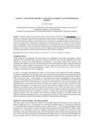
It is important to note that the concentration pattern is often irregular
for the Kincaid experiment – high and low concentrations may occur
intermittently along an arc. Figure 2 shows an example. Therefore it is
often difficult to determine a representative maximum concentration
along a crosswind arc of monitors. Further, there may be gaps in the
monitoring arcs. Therefore, a variable has been assigned to each
monitoring arc, indicating how reliable the arc-wise maximum should
be considered. This quality indicator has been assigned by Earth Tech
on the basis of manual inspection of the geographical patterns of
concentration distribution. The criteria for assigning the indicator are
shown in Table 1.
12
0
43
0
0
0
37
74
90 106 6 9
0
10
0
0
0
0
0
0
0
22
0
8
0
104
0 0 0 23 15 0 110 119
0
238
0
0
0 0
6 0
North-South (km)
6
4
0
0
0
0
14
0
0
0
0
0
0
0
38
0
0
0
86 83
52 63 92
20
0
7
0
0
0
0
0
0
0
0
0
0
0
0
0
NP
NP
0
2
000 0 00 00 0 00 0
0
0
00
12
130
0
0
0
NP
0
0 0 0
NP
0
0
0
0
NP
0
6RXUFH
NP
-6 -4 -2 0
2 4 6
East-West (km)
Figure 2 Geographical distribution of measured concentrations at Kincaid, 22 May 1981, 10-11
hours. Values are in ppt, and the arcwise maxima are enclosed in circles.
The complete set of tracer measurements at all monitors is distributed
in the file SF6_ALL.DAT. The format of this file is a bit awkward, but
in the folder *UDSKHUBWRROV there is software capable of extracting
information from it (See Chapter 9). An alternative is to use data in
the ASTM package (see Section 3.2 with FAQ).
.
20

Table 1 The file QUAL.TXT contains the following explanation of quality indicator (QUAL) for Kincaid and Indianapolis.
The indicator variable has values from 0 to 3, indicating the following:
0 This value should clearly be disregarded (examples: the plume obviously missed the monitors; the arc is
only a continuation of a neighbouring arc).
1 This value is most probably not the maximum value (examples: there are gaps in the monitoring arc; the
observed maximum is isolated; there is no smooth variation from one arc to the next; the maximum is on the edge
of the arc).
2 A maximum is identified, but the true value may well be different (examples: the concentration pattern is
irregular; there are only 2 or 3 monitors impacted; the plume is near the edge of the arc).
Note: Also, arcs where the observed maximum is essentially zero, but where there is evidence that a plume is
present aloft, have been categorized in this group.
3 A relatively well-defined maximum is observed, which is continuous in space, is away from the edge of the
monitoring arc, and is not irregular or isolated.
It is recommended that you use data with a quality indicator of 2 or 3 in your analyses. Note that observations
with QUAL=3 are biased in the sense that they are never zero.
5.1.4 Data files
"Hour" indicates "end of the hour" for time-averaged parameters.
Thus, 10 means an average over the period between 9 and 10 Central
Standard Time. CST is equivalent to GMT-6.
The following files are supplied in the LQFDLG folder:
DISTM_K.DAT Distances to arcs with values of max. conc.
EMISSION.DAT Emission data for all hours, not just sampling hours.
GEO_KIN.TXT Info on geographical coordinates.
MET_K1-L.DAT Meteorological data; ’long’ (continuous) period
MET_K1.DAT Meteorological data; tracer hours
MET_K2-L.DAT More met. parameters
MET_K2.DAT -
MET_K3-L.DAT -
MET_K3.DAT -
MISC_KIN.DAT Miscellaneous data
OUTLIERS.TXT Information on outliers (changes to original data)
PAR_KIN.TXT Overview of parameters and missing data.
QUAL.TXT Explanation of quality indicator
RAWIN.DAT Routine radiosonde data
SF6_ALL.DAT SF 6
data, all monitors
SF6_KIN.DAT SF 6
data, arc-wise maxima
There are corresponding pairs of files such as MET_K1.DAT and
MET_K1-L.DAT. The ’L’ files are ’long’, and include meteorological
information for the hours between tracer experiments. They have
been included to permit modellers to run met preprocessor requiring
continuous periods of data.
The tables on the next pages yield an overview of the variables
contained in the data sets.
5.1.5 Points to be noted
A summary of some potential pitfalls when using data is given
below:
• The derived meteorological parameters, u *
, w *
, L and h pred
, should
be used with care or replaced.
• and are suspected to be unreliable. According to Steve
w v
Hanna, there were many problems with Gill data, and use of
w
them may severely degenerate modelling results.
Also, according to results for one specific model shown at the
workshop in Manno, the effect of choosing observed values of
v
– as opposed to computed values – resulted in predictions of the
21

maximum concentration for the entire data set which were factor
of three larger than otherwise.
• It is recommended to use data with a quality indicator of 2 or 3
when analyzing model behaviour. One point is important to be
aware of: observations with QUAL=3 are biased in the sense that
they are never zero.
5.1.6 Additional information
The data distributed constitute only a small fraction of the wide
variety of variables collected during the campaign. A large number of
reports concerning the Kincaid experiment have been published by
EPRI. Therefore, if you wish to analyze certain questions in further
detail, you may want to request some of these reports from EPRI (see
the list of addresses at the end of the chapter with references..
Also, please note that a piece of recommended reading concerning
the Kincaid experiment is the paper Hybrid Plume Dispersion Model
(HPDM) Development and Evaluation by Hanna and Paine (1989). It
gives a brief description of the layout of the Kincaid experimental
campaign.
See the list of references and the list of addresses in the back for
details.
22

Table 2 Contents of the file PAR_KIN.TXT
Basic parameters:
Parameters supplied in the distributed files from Kincaid
=========================================================
FILE NAMES
3 files with each 2040 obs.: MET_K1-L.DAT MET_K3-L.DAT
MET_K2-L.DAT
4 files with each 171 obs.: MISC_KIN.DAT MET_K1.DAT MET_K2.DAT MET_K3.DAT
1 file with 1284 obs.: SF6_KIN.DAT
YR Year + + + + +
MO Month + + + + +
DY Day + + + + +
HR Hour (end of hour; GMT-6) + + + + +
Observed meteorological parameters:
PRES Pressure (mb) +
NET Net radiation (W/m2) +
TOT Total radiation (W/m2) +
DP100 Dew-point temperature at 100 m (K) +
T100 Temperature at 100 m (K) +
T50 Temperature at 50 m (K) +
T10 Temperature at 10 m (K) +(*1) +
ZI Mixing height, observed (m) + +
DTHDZ Pot. temp. grad. between 100-50 m (K/m) + +
WS100 Wind speed at 100 m (m/s) + +
WS50 Wind speed at 50 m (m/s) +
WS30 Wind speed at 30 m (m/s) +
WS10 Wind speed at 10 m (m/s) +(*1) +
WD100 Wind direction at 100 m (deg.) +(*1) +
WD50 Wind direction at 50 m (deg.) +
WD30 Wind direction at 30 m (deg.) +
WD10 Wind direction at 10 m (deg.) +
SWD100 Sigma WD100 (deg.) +
SWD50 Sigma WD50 (deg.) +
SWD30 Sigma WD30 (deg.) +
SWD10 Sigma WD10 (deg.) +
SIGW Sigma of vertical velocity at 100 m (m/s) + +
SIGV Sigma of cross-wind speed at 100 m (m/s) + +
FLAG (*2) +
CEILNWS Ceiling (100’s of feet); -1=unlimited +
DPNWS Dew-point temp. (F) +
WDNWS Wind direction (deg.) +
WSNWS Wind speed (knots) +
PNWS Pressure (inch. Hg) +
TNWS Temperature (F) +
NNWS Cloud cover (1/10) +
PRECNWS Precipitation (mm) +
Derived parameters:
ZIPRE Predicted mixing height (m) +
UST Friction velocity (m/s) +
WST Convective velocity (m/s) +
L Monin-Obukhov length (m) +
TURNER Turner stability class (based on NWS data) +
Tracer parameters:
Q Emission rate (g/s) + +
TQ Gas temp. (K) +
VSQ Gas exit velocity (m/s) +
ARCMAX Max. conc. (ug/m3) at DIST (*3) +
DIST Distance (km) to arc of monitors +
AZMAX Direction (deg.) to ARCMAX +
ARCMAX/Q Conc normalized by emission, times 10**9 (s/m3 10**(-9)) +
QUAL Quality indicator for ARCMAX +
(*1): 5-6 observations are substituted with converted NWS observations.)
(*2): Value of flag describes which of the parameters T10, WS10 or WD100 are substituted.
For each of the substitutions FLAG is added the value 1, 2 resp. 4 (no subs. FLAG=0).)
(*3): Converted from ppt by multiplying with 1.758*p/T)
The file DISTM_K.DAT is meant as a help for deciding at which distances computations
should be performed (where SF6 was measured). 12 different distance values appear in
the data set.
Parametre
Units
DISTM_K
YR Year +
MO Month +
DY Day +
HR Hour, (GMT-6) +
NUARCM Number of arcs with values of max. conc. ARCMAX +
DM1 Distances (km) to arcs with +
DM2 values of ARCMAX +
... DM12 +
23

Table 3
Contents of the file PAR_KIN.TXT (continued)
Number of missing parameters and their dummy values in the distributed files from Kincaid.
FILE NAMES
Para- Dummy MISC_KIN.DAT MET_K1.DAT MET_K1-L.DAT MET_K2.DAT MET_K2-L.DAT MET_K3.DAT MET_K3-L.DAT SF6_KIN.DAT
meters value
YR - 0 0 0 0 0 0 0 0
MO - 0 0 0 0 0 0 0 0
DY - 0 0 0 0 0 0 0 0
HR - 0 0 0 0 0 0 0 0
PRES -999 5 62
NET -999 8 202
TOT -999 8 379
DP100 -999 52 370
T100 -999 8 205
T50 -999 8 205
T10 -999 0 5 37
ZI -999 6 6 906
DTHDZ -9.9999 8 8 239
WS100 -999 6 6 112
WS50 -999 9 206
WS30 -999 6 40
WS10 -999 0 6 42
WD100 -999 0 5 44
WD50 -999 8 207
WD30 -999 8 208
WD10 -999 5 40
SWD100 -999 6 190
SWD50 -999 6 189
SWD30 -999 6 189
SWD10 -999 6 189
SIGW -9.99 18 18 461
SIGV -9.99 9 9 885
FLAG -
CEILNWS - 0 0
DPNWS - 0 0
WDNWS - 0 0
WSNWS - 0 0
PNWS - 0 0
TNWS - 0 0
NNWS - 0 0
PRECNWS - 0 0
ZIPRE - 0
UST - 0
WST - 0
L - 0
TURNER - 0
Q - 0 0
TQ - 0
VSQ - 0
DIST - 0
ARCMAX - 0
AZMAX -999 355
ARCMAX/Q - 0
QUAL - 0
Notes on parameters:
--------------------
The derived meteorological parameters have been included for reference.
They are computed using one of many possible methods and their inclusion
in the data set does not indicate a recommendation of their use.
It is recommended that modellers use their own processing methods.
Measured values of SIGW and SIGV are not to be considered reliable.
The Turner stability class has been computed based on NWS data. It is
included for reference; it is computed according to the original paper by
Turner: J. Appl. Met., (1964) 3., p.83 (this is the case also for
Copenhagen and Lillestrom data).
Be careful about units when using NWS data - they differ from the
European units!
The frequency distribution of the quality index for tracer arc-hours is as follows
QUAL Frequency
------------------
0 442
1 256
2 248
3 338
All: 1284
24

Table 4 Samples of the most important data files from Kincaid.
MISC_KIN.DAT
YR MO DY HR ZI ZIPRE DTHDZ T10 WS10 WS100 WD100 SIGV SIGW UST WST L TURNER Q TQ VSQ FLAG
80 4 20 14 2076 2288 -9.9999 298.4 2.7 5.8 281 -9.99 -9.99 0.30 2.65 -8.6 4 10.2 416.0 14.6 0
80 4 20 15 2092 2313 -9.9999 298.4 2.9 5.8 302 -9.99 -9.99 0.31 2.53 -11.2 4 8.2 416.0 14.6 0
80 4 20 16 2104 2333 -9.9999 298.4 2.5 6.3 308 -9.99 -9.99 0.28 2.31 -9.9 4 8.4 416.0 15.0 0
80 4 25 12 893 1156 -0.0022 284.2 2.0 2.3 57 1.35 0.84 0.22 1.95 -3.9 2 11.2 432.0 29.6 0
80 4 25 13 1032 1332 -0.0022 285.2 2.1 2.3 52 0.49 0.90 0.22 1.95 -4.8 1 11.2 432.0 29.2 0
80 4 25 14 1175 1575 -0.0022 286.2 3.0 3.3 53 1.11 0.77 0.28 2.05 -10.4 3 11.3 432.0 29.6 0
80 4 25 15 1355 1753 -0.0022 286.6 2.1 2.4 29 1.23 0.71 0.25 2.19 -6.3 3 11.1 432.0 29.9 0
80 4 25 16 1539 1768 -0.0022 287.3 5.1 -999.0 42 -9.99 0.80 0.51 1.92 -84.7 3 11.3 432.0 30.0 2
80 4 25 17 1545 1774 -0.0022 287.7 2.3 2.8 31 0.53 0.62 0.23 1.39 -20.9 4 10.7 432.0 30.3 0
80 5 1 16 1300 1932 -0.0002 290.8 3.5 3.9 15 1.01 0.74 0.37 2.17 -23.5 3 11.5 441.0 27.9 0
MET_K1.DAT
YR MO DY HR PRES NET TOT DP100 T100 T50 T10 ZI DTHDZ
80 4 20 14 1000.0 -999.0 -999.00 279.5 -999.0 -999.0 298.4 2076 -9.9999
80 4 20 15 999.7 -999.0 -999.00 278.8 -999.0 -999.0 298.4 2092 -9.9999
80 4 20 16 999.7 -999.0 -999.00 278.8 -999.0 -999.0 298.4 2104 -9.9999
80 4 25 12 995.4 503.8 773.84 271.6 283.0 283.6 284.2 893 -0.0022
80 4 25 13 995.0 439.0 662.27 272.0 284.0 284.6 285.2 1032 -0.0022
80 4 25 14 994.7 432.9 685.54 272.3 284.8 285.4 286.2 1175 -0.0022
80 4 25 15 994.0 368.0 572.16 272.6 285.5 286.1 286.6 1355 -0.0022
80 4 25 16 993.5 250.7 415.56 272.5 286.2 286.8 287.3 1539 -0.0022
80 4 25 17 993.2 94.3 214.55 272.6 286.6 287.2 287.7 1545 -0.0022
80 5 1 16 994.5 331.3 545.19 278.6 289.7 290.2 290.8 1300 -0.0002
80 5 1 17 994.3 152.7 280.01 278.2 290.3 290.8 291.3 1743 -0.0002
80 5 1 18 994.2 60.5 179.78 278.1 290.5 291.0 291.6 1840 -0.0002
MET_K1-L.DAT
YR MO DY HR PRES NET TOT DP100 T100 T50 T10 ZI DTHDZ
80 4 14 1 988.1 -999.0 -999.00 271.5 -999.0 -999.0 272.8 154 -9.9999
80 4 14 2 984.8 -999.0 -999.00 269.1 -999.0 -999.0 272.8 -999 -9.9999
80 4 14 3 982.7 -999.0 -999.00 270.8 -999.0 -999.0 273.5 -999 -9.9999
80 4 14 4 981.4 -999.0 -999.00 273.5 -999.0 -999.0 274.4 -999 -9.9999
80 4 14 5 980.0 -999.0 -999.00 272.8 -999.0 -999.0 274.4 -999 -9.9999
80 4 14 6 979.3 -999.0 -999.00 272.4 -999.0 -999.0 273.5 -999 -9.9999
80 4 14 7 978.7 -999.0 -999.00 272.4 -999.0 -999.0 273.5 -999 -9.9999
80 4 14 8 977.3 -999.0 -999.00 272.4 -999.0 -999.0 273.5 -999 -9.9999
80 4 14 9 976.0 -999.0 -999.00 272.4 -999.0 -999.0 273.5 -999 -9.9999
80 4 14 10 975.3 -999.0 -999.00 271.9 -999.0 -999.0 273.5 -999 -9.9999
80 4 14 11 975.3 -999.0 -999.00 271.5 -999.0 -999.0 273.5 -999 -9.9999
80 4 14 12 976.0 -999.0 -999.00 271.5 -999.0 -999.0 273.5 -999 -9.9999
80 4 14 13 976.6 -999.0 -999.00 271.5 -999.0 -999.0 273.5 -999 -9.9999
80 4 14 14 978.0 -999.0 -999.00 271.5 -999.0 -999.0 272.8 -999 -9.9999
80 4 14 15 978.0 -999.0 -999.00 271.1 -999.0 -999.0 272.8 -999 -9.9999
80 4 14 16 980.0 -999.0 -999.00 271.1 -999.0 -999.0 272.8 -999 -9.9999
80 4 14 17 980.7 -999.0 -999.00 271.1 -999.0 -999.0 272.8 -999 -9.9999
80 4 14 18 981.4 -999.0 -999.00 271.1 -999.0 -999.0 272.8 -999 -9.9999
80 4 14 19 982.7 -999.0 -999.00 271.1 -999.0 -999.0 272.8 -999 -9.9999
80 4 14 20 983.4 -999.0 -999.00 271.5 -999.0 -999.0 272.8 -999 -9.9999
80 4 14 21 984.1 -999.0 -999.00 271.5 -999.0 -999.0 272.8 -999 -9.9999
80 4 14 22 984.1 -999.0 -999.00 271.5 -999.0 -999.0 272.8 -999 -9.9999
80 4 14 23 984.8 -999.0 -999.00 271.5 -999.0 -999.0 272.8 -999 -9.9999
80 4 14 24 984.8 -999.0 -999.00 271.5 -999.0 -999.0 272.8 -999 -9.9999
80 4 15 1 984.8 -999.0 -999.00 271.5 -999.0 -999.0 273.5 -999 -9.9999
80 4 15 2 984.8 -999.0 -999.00 272.4 -999.0 -999.0 272.8 -999 -9.9999
MET_K2.DAT
YR MO DY HR WS100 WS50 WS30 WS10 WD100 WD50 WD30 WD10 SWD100 SWD50 SWD30 SWD10 SIGW SIGV
80 4 20 14 5.8 -999.0 5.8 2.7 281 -999 -999 302 -999.00 -999.00 -999.00 -999.00 -9.99 -9.99
80 4 20 15 5.8 -999.0 6.3 2.9 302 -999 -999 319 -999.00 -999.00 -999.00 -999.00 -9.99 -9.99
80 4 20 16 6.3 -999.0 6.3 2.5 308 -999 -999 313 -999.00 -999.00 -999.00 -999.00 -9.99 -9.99
80 4 25 12 2.3 2.2 2.2 2.0 57 49 46 29 47.11 59.17 65.37 70.49 0.84 1.35
80 4 25 13 2.3 2.4 2.3 2.1 52 54 53 46 12.42 14.81 15.91 27.52 0.90 0.49
80 4 25 14 3.3 3.3 3.3 3.0 53 55 58 53 20.39 22.98 22.65 32.17 0.77 1.11
80 4 25 15 2.4 2.4 2.3 2.1 29 27 34 20 35.22 47.36 55.78 65.40 0.71 1.23
80 4 25 16 -999.0 -999.0 -999.0 -999.0 42 40 41 34 33.53 31.72 32.16 40.79 0.80 -9.99
80 4 25 17 2.8 2.6 2.5 2.3 31 27 26 16 11.02 21.18 26.15 29.04 0.62 0.53
80 5 1 16 3.9 4.1 4.0 3.5 15 16 16 7 15.29 15.41 16.36 16.56 0.74 1.01
80 5 1 17 4.0 4.0 3.9 3.4 21 21 19 11 8.61 7.26 8.21 7.59 0.53 0.59
80 5 1 18 3.8 3.7 3.5 3.0 33 34 33 25 11.97 10.94 11.67 12.03 0.45 0.78
80 5 1 19 4.0 3.8 3.4 2.8 47 46 44 36 3.69 3.73 3.71 4.33 0.22 0.26
80 5 1 20 3.2 2.7 2.2 1.4 67 63 64 60 14.20 12.31 13.28 20.20 0.13 0.77
80 5 1 21 2.4 2.2 1.9 0.9 133 137 133 147 14.92 18.86 23.32 28.54 0.09 0.60
80 5 4 7 4.9 2.9 1.7 1.0 323 333 339 326 5.40 3.18 3.71 21.19 0.06 0.46
80 5 4 8 4.6 2.3 2.0 1.7 331 337 337 336 1.38 3.20 2.92 8.01 0.19 0.11
80 5 4 9 3.0 2.8 2.8 2.5 340 343 342 337 3.86 3.57 4.40 4.86 0.37 0.20
MET_K3.DAT
YR MO DY HR CEILNWS DPNWS WDNWS WSNWS PNWS TNWS NNWS PRECNWS
80 4 20 14 -1 55 29 12 29.97 80 2 0.0
80 4 20 15 -1 52 29 14 29.97 81 3 0.0
80 4 20 16 -1 51 32 12 29.94 80 2 0.0
80 4 25 12 -1 35 30 6 29.97 57 3 0.0
80 4 25 13 -1 39 20 4 29.94 59 2 0.0
80 4 25 14 -1 41 1 8 29.94 60 3 0.0
80 4 25 15 -1 41 31 10 29.91 62 3 0.0
80 4 25 16 -1 41 1 10 29.91 61 3 0.0
80 4 25 17 -1 40 3 10 29.91 60 2 0.0
80 5 1 16 -1 50 4 8 29.94 68 3 0.0
80 5 1 17 -1 50 3 8 29.94 68 3 0.0
SF6_KIN.DAT
YR MO DY HR ARCMAX DIST AZMAX Q ARCMAX/Q QUAL
80 4 20 14 0.748 3.0 92 10.2 73.4 3
80 4 20 14 0.218 5.0 117 10.2 21.4 1
80 4 20 14 0.216 7.0 94 10.2 21.2 1
80 4 20 14 0.138 10.0 95 10.2 13.6 1
80 4 20 14 0.210 15.0 131 10.2 20.6 1
80 4 20 14 0.084 20.0 57 10.2 8.3 1
80 4 20 15 0.442 3.0 83 8.2 53.9 3
80 4 20 15 0.249 5.0 120 8.2 30.3 3
25

Table 5 Format of RAWIN.DAT (radiosonde data).
26

5.2 Copenhagen
5.2.1 Experimental set-up
The experiments in question took place in the Northern part of
Copenhagen in 1978-79. A full description can be found in Gryning
(1981; available on request). A shorter description is found in a paper
by Gryning and Lyck (1984; available from Helge Rørdam Olesen on
request). A comprehensive data report is available electronically
(Gryning and Lyck, 2002).
The dispersion experiments were carried out under neutral and
unstable conditions. The tracer (SF 6
) was released without buoyancy
from a tower at a height of 115 m, and collected at ground-level
positions in up to three crosswind series of tracer sampling units,
positioned 2-6 km from the point of release. The site was mainly
residential having a roughness length of 0.6 m.
For all runs during the experiment, the crosswind profiles of tracer
concentrations were well determined, thus making a relatively accurate
estimate of crosswind integrated concentration possible. The
maximum concentrations given in the data set is the highest observed
concentration along each arc.
The release took place in the suburb of Gladsaxe, latitude 55.735 N,
longitude 12.494 E; the height of terrain is 49 m a.m.s.l. The tracer
sampling units were mounted at lampposts at a height of 2-3 meters
above the ground.
Figure 3 The experimental site in Copenhagen. A thick line indicates the
coast of the straight of Øresund. Tracer sampling unit positions available for
the experiments are indicated by circles. Not all positions were used for an
experiment. Typically, 20 sampling units were used in each arc, and the
units were deployed according to meteorological conditions.
27

5.2.2 Meteorological data
The meteorological measurements performed during the experiments
included three-dimensional wind velocity fluctuations at the height
of release. Much emphasis was put into the measurements at the
release height (Gryning and Thomson, 1979). These measurements
comprised u, v
and w
. It is recommended to make use of these
measurements (cf. Gryning and Tassone, 1994). The temperature and
wind speed profile along the mast was taken from routine
measurements. The mixing height was determined from the daily
radio sounding at Copenhagen, which was carried out around the
time of tracer sampling.
In the revised data set, the values of u *
, L and heat flux have been
determined using a standard meteorological preprocessor (in an
implementation described by Sozzi and Fraternali, 1994). Two levels
of temperature and one level of wind speed were used (not researchgrade
data). The computed heat fluxes etc. may be influenced by very
local effects; in one case in particular, the heat flux was much larger
than expected.
5.2.3 Points to be noted
The tracer monitoring arcs were in general placed at distances where
the concentration was decreasing, i.e., the maximum was closer to the
source than any of the arcs.
It is observed (Gryning and Tassone, 1994) that measured values of
are smaller than predictions by theory.
w
The computed heat flux values may not be representative for a
greater area.
5.2.4 Additional information
It is possible upon request to obtain supplementary meteorological
data for the time before the measuring periods.
Please note that a comprehensive data report on the Copenhagen
data set is available through the Web (Gryning and Lyck, 2002) .
28

Table 6 Contents of the file PAR_CPH.TXT
Parameters supplied in the distributed files from Copenhagen
============================================================
Basic parameters:
YR Year
MO Month
DY Day
HRS Time start of period, (GMT+1). Example: 1317 means 13.17
HRE Time end of period, (GMT+1)
Observed meteorological parameters:
W10 Wind speed at 10 m (m/s)
W60 Wind speed at 60 m (m/s)
W115 Wind speed at 115 m (m/s)
T2 Temperature at 2 m (deg. K)
T40 Temperature at 40 m (deg. K)
T120 Temperature at 120 m (deg. K)
SIGV Sigma of cross-wind speed at 115 m (m/s)
SIGW Sigma of vertical velocity at 115 m(m/s)
ZI Mixing height, observed (m)
NCLD Fractional cloud cover (EIGHTS!)
CEIL Height to lowest cloud (m)
Derived meteorological parameters:
UST Friction velocity from profile (m/s)
L Monin-Obukhov length (m)
HF Heat flux (W/m2)
TURNER Turner stability class according to Turner (1964)
Tracer release parameters:
DIST Distance (km) to arc of monitors
Q Emission rate (g/s)
SIGY Sigma-y (m) at DIST
CY Cross-wind integ. conc. (ug/m2) at DIST
CY/Q CY normalized by emission, times 10**6 (s/m2 10**(-6))
ARCMAX Max. conc. (ug/m3) at DIST
ARCMAX/Q Conc normalized by emission, times 10**9 (s/m3 10**(-9))
HS Tracer release height (m)
NUARC Number of arcs for an experiment
D1-D3 Distance (km) to arcs for an experiment
Notes on parameters:
--------------------
Measured values of SIGV and SIGW are considered more reliable than those
deduced from profile measurements.
The values of T2, W10 etc. have been formed as the average of 6 10-minute
averages.
HF, UST and L have been determined using measurements from a met tower
(two levels of temperature, one level of wind speed: T2, T40 and W10).
A roughness length of 0.6 m has been assumed.
For the processing, the subroutine PBL_1 of the software library
PBL_MET (described by Sozzi and Fraternali, 1994) has been used.
Turner stability class is computed according to the original paper by Turner:
J. Appl. Met., (1964) 3., 83.
Changes compared to the data set distributed for the Manno workshop:
--------------------------------------------------------------------
The following parameters have been included:
W60, T120, NCLD, CEIL, CY/Q, ARCMAX/Q
The parameter P (Pasquill class) has been omitted, and instead a Turner
stability class has been included.
The derived values of UST, L and HF have been determined using a standard
preprocessor, whereas they were formerly determined by a manual method.
29

Table 7 The full contents of files from Copenhagen.
MET_CPH.DAT
Revised data set for Copenhagen. Version from May 94, based on 6 10-min values.
YR MO DY HRS HRE W10 W60 W115 T2 T40 T120 SIGV SIGW ZI NCLD CEIL UST L HF TURNER
78 09 20 1317 1417 2.1 999.0 3.4 285.5 284.2 283.4 0.98 0.83 1980 7 7500 .36 -37 116. 3
78 09 26 1140 1240 4.9 999.0 10.6 288.7 287.5 286.6 1.39 1.07 1920 6 6000 .73 -292 120. 4
78 10 19 1213 1313 2.3 999.0 5.0 285.6 284.6 283.9 0.85 0.68 1120 5 480 .38 -71 69. 4
78 11 03 1320 1420 2.5 999.0 4.6 284.8 284.0 283.3 0.47 0.47 390 4 3600 .38 -133 39. 3
78 11 09 1330 1430 3.1 999.0 6.7 285.5 284.9 284.2 0.77 0.71 820 7 750 .45 -444 19. 4
79 04 30 1302 1402 7.2 11.7 13.2 280.1 278.6 277.6 2.26 1.33 1300 5 750 1.05 -432 242. 4
79 06 27 1245 1345 4.1 7.2 7.6 292.2 290.4 289.5 1.61 0.87 1850 6 2400 .64 -104 227. 3
79 07 06 1250 1350 4.2 10.6 9.4 293.8 290.9 289.9 1.35 0.72 810 5 6000 .69 -56 530. 3
79 07 19 1215 1315 5.1 9.0 10.5 289.8 288.5 287.5 1.71 0.98 2090 6 600 .75 -289 134. 4
SF6_CPH.DAT
YR MO DY HRS HRE DIST Q SIGY CY CY/Q ARCMAX ARCMAX/Q HS
78 09 20 1317 1417 1.90 3.2 254 2074 648. 3.360 1050.0 115
78 09 20 1317 1417 3.70 3.2 444 739 231. 0.685 214.1 115
78 09 26 1140 1240 2.10 3.2 329 1722 538. 3.152 985.0 115
78 09 26 1140 1240 4.20 3.2 438 944 295. 0.906 283.1 115
78 10 19 1213 1313 1.90 3.2 184 2624 820. 5.226 1633.1 115
78 10 19 1213 1313 3.70 3.2 283 1990 622. 2.544 795.0 115
78 10 19 1213 1313 5.40 3.2 404 1376 430. 1.203 375.9 115
78 11 03 1320 1420 4.00 2.3 301 2682 1166. 3.613 1570.9 115
78 11 09 1330 1430 2.10 3.2 185 2150 672. 3.875 1210.9 115
78 11 09 1330 1430 4.20 3.2 279 1869 584. 2.317 724.1 115
78 11 09 1330 1430 6.10 3.2 376 1590 497. 1.520 475.0 115
79 04 30 1302 1342 2.00 3.1 -999 1228 396. 2.306 743.9 115
79 04 30 1302 1342 4.20 3.1 -999 688 222. 1.045 337.1 115
79 04 30 1302 1342 5.90 3.1 -999 567 183. 0.539 173.9 115
79 06 27 1245 1345 2.00 2.4 290 1608 670. 2.275 947.9 115
79 06 27 1245 1345 4.10 2.4 595 780 325. 0.629 262.1 115
79 06 27 1245 1345 5.30 2.4 786 535 223. 0.276 115.0 115
79 07 06 1250 1350 1.90 3.0 190 1248 416. 2.928 976.0 115
79 07 06 1250 1350 3.60 3.0 402 606 202. 0.792 264.0 115
79 07 06 1250 1350 5.30 3.0 580 456 152. 0.294 98.0 115
79 07 19 1215 1318 2.10 3.3 236 1511 458. 2.812 852.1 115
79 07 19 1215 1318 4.20 3.3 460 1026 311. 0.878 266.1 115
79 07 19 1215 1318 6.00 3.3 623 855 259. 0.653 197.9 115
DIST_C.DAT
YR MO DY HRE NUARC D1 D2 D3
78 09 20 1417 2 1.90 3.70
78 09 26 1240 2 2.10 4.20
78 10 19 1313 3 1.90 3.70 5.40
78 11 03 1420 1 4.00
78 11 09 1430 3 2.10 4.20 6.10
79 04 30 1402 3 2.00 4.20 5.90
79 06 27 1345 3 2.00 4.10 5.30
79 07 06 1350 3 1.90 3.60 5.30
79 07 19 1318 3 2.10 4.20 6.00
30

5.3 Lillestrøm data
5.3.1 Experimental set-up
The tracer experiments of concern here took place in the town of
Lillestrøm (near Oslo), Norway in 1987. They were performed by the
Norwegian Institute of Air Research (NILU) which has put the data at
our disposal.
A detailed description is given by Haugsbakk and Tønnesen (1989;
available on request). A shorter description is found in the paper by
Grønskei (1990).
Release from a 36 m mast.
15-minute sampling
The experiments were carried out in a flat residential area with 6-10
m high buildings and trees. A tracer system was used in which SF 6
was released from a mast 36 m above the ground. Each experiment
consisted of two sequential 15-min periods. Thus, the sampling
period is shorter than for the other experiments considered at the
workshop.
The meteorological measurements were carried out along the 36 m
high mast.
Sonic anemometer measurements were processed to give 10 min
average values for wind speed and wind directions at the 10 m level.
Further, covariances were determined between velocity components,
and between velocity components and temperature fluctuations.
Norwegian winter: Snowcovered
ground, low sun
The temperature during the tracer experiments was low ( - 20(
Celsius), and the ground was snow-covered. The sun was above the
horizon, but at a very low angle. The surface roughness was about 0.5
m.
Generally, the vertical temperature profiles in the lowest 100 m
showed an inversion (Haugsbakk and Tønnesen, 1989).
For all runs during the experimental campaign, the crosswind
profiles of tracer concentrations were well determined, thus making a
relatively accurate estimate of crosswind integrated concentration
possible. The maximum concentrations given in the data set is the
highest observed concentration along each arc.
Geographical coordinates for the position of release are: latitude
59.889 N, longitude 11.051 E; the height of terrain is 110 m a.m.s.l.
5.3.2 Points to be noted
Note that for Lillestrøm data, the averaging period is only 15 minutes
for the tracer data. Concentration averages taken over longer time
will tend to be smaller than those registered, due to meandering.
There was generally very light wind during the experiments.
u *
was recorded as zero for the experiment with the highest concentrations.
31

In the data set, stability category has been computed based upon the
original method by Turner (1964). This is consistent with the method
used for the other data sets, but it does not very well take account of
Norwegian winter conditions with snow-covered ground.
Table 8
Contents of the file PAR_LIL.TXT
Parameters supplied in the distributed files from Lillestrom
============================================================
Note: the last observation in the data set was performed in
conditions with VERY low wind speed (0.2 m/s at a height of 36 m).
L was not determined.
Basic parameters:
YR Year
MO Month
DY Day
HRS Time start of period, (GMT+1). Example: 1317 means 13.17
HRE Time end of period, (GMT+1)
Observed meteorological parameters:
WS10 Wind speed at 10 m sonic-anemometer (m/s)
WS36 Wind speed at 36 m cup-anemometer (m/s); four values are missing, i.e. -99.9
T10 Temperature at 10 m (deg. K)
DT Temperature difference 36-10 m (deg. K)
SIGV Sigma of cross-wind speed at 10 m, sonic-anemometer (m/s)
SIGW Sigma of vertical velocity at 10 m, sonic-anemometer (m/s)
ZI Mixing height - missing, i.e. -999
NCLD Fractional cloud cover (EIGHTS!)
CEIL Height to lowest cloud (m); -1=unlimited
UST Friction velocity at 10 m, sonic anemometer (m/s)
L Monin-Obukhov length, sonic anemometer (m)
Derived meteorological parameters:
TURNER Turner stability class according to Turner (1964)
Tracer release parameters:
DIST Distance (km) to arc of monitors
Q Emission rate (g/s)
SIGY Sigma-y (m) at DIST
CY Cross-wind integ. conc. (ug/m2) at DIST
CY/Q CY normalized by emission, times 10**6 (s/m2 10**(-6))
ARCMAX Max. conc. (ug/m3) at DIST
ARCMAX/Q Conc normalized by emission, times 10**9 (s/m3 10**(-9))
HS Tracer release height (m)
NUARC Number of arcs for an experiment
D1-D3 Distance (km) to arcs for an experiment
Notes on parameters:
--------------------
Turner stability class is computed according to the original paper by Turner:
J. Appl. Met., (1964) 3., 83 (thus, there is no provision for the snow
cover on the ground).
Changes compared to the data set distributed for the Manno workshop:
--------------------------------------------------------------------
The following parameters have been included:
NCLD, CEIL, CY/Q, ARCMAX/Q, DT
The parameter P (Pasquill class) has been omitted, and instead a Turner
stability class has been included.
Four values of W36 are now considered missing.
32

Table 9 The full contents of data files from Lillestrøm.
MET_LIL.DAT
YR MO DY HRS HRE W10 W36 T10 DT SIGV SIGW ZI NCLD CEIL UST L TURNER
87 01 10 930 945 2.1 4.4 247.7 -0.1 0.62 0.47 -999 0 -1 0.374 235 4
87 01 10 945 1000 1.7 3.6 247.7 -0.2 0.54 0.42 -999 0 -1 0.283 130 3
87 01 12 930 945 1.7 3.0 252.7 1.3 0.32 0.22 -999 0 -1 0.173 27 3
87 01 12 945 1000 1.6 3.1 252.7 1.3 0.32 0.22 -999 0 -1 0.173 41 3
87 01 17 1000 1015 0.9 -99.9 252.0 1.5 0.24 0.10 -999 0 -1 0.224 -1601 3
87 01 17 1015 1030 0.5 -99.9 252.0 1.3 0.17 0.10 -999 0 -1 0.100 188 3
87 02 09 1000 1015 0.5 -99.9 260.4 0.2 0.17 0.17 -999 4 3050 0.100 -8.1 3
87 02 09 1015 1030 0.4 -99.9 260.4 0.5 0.22 0.14 -999 4 3050 0.000 -9999 3
SF6_LIL.DAT
YR MO DY HRS HRE DIST Q SIGY CY CY/Q ARCMAX ARCMAX/Q HS
87 01 10 930 945 0.160 0.102 65 1082 10608. 7.6 74510. 36
87 01 10 930 945 0.490 0.102 129 1029 10088. 4.8 47059. 36
87 01 10 930 945 0.810 0.102 144 1049 10284. 3.7 36275. 36
87 01 10 945 1000 0.140 0.102 54 1161 11382. 8.3 81373. 36
87 01 10 945 1000 0.440 0.102 132 1337 13108. 5.2 50980. 36
87 01 10 945 1000 0.820 0.102 237 1486 14569. 3.4 33333. 36
87 01 12 930 945 0.150 0.102 49 1060 10392. 11.1 108824. 36
87 01 12 930 945 0.300 0.102 68 437 4284. 2.7 26471. 36
87 01 12 930 945 0.460 0.102 115 633 6206. 2.3 22549. 36
87 01 12 945 1000 0.160 0.102 52 988 9686. 8.6 84314. 36
87 01 12 945 1000 0.300 0.102 58 741 7265. 5.8 56863. 36
87 01 12 945 1000 0.440 0.102 113 774 7588. 2.8 27451. 36
87 01 17 1000 1015 0.150 0.102 41 637 6245. 6.9 67647. 36
87 01 17 1000 1015 0.470 0.102 98 484 4745. 3.3 32353. 36
87 01 17 1000 1015 0.900 0.102 134 2732 26784. 7.6 74510. 36
87 01 17 1015 1030 0.150 0.102 69 256 2510. 1.7 16667. 36
87 01 17 1015 1030 0.490 0.102 79 1327 13010. 6.2 60784. 36
87 01 17 1015 1030 0.900 0.102 131 1138 11157. 5.8 56863. 36
87 02 09 1000 1015 0.190 0.102 55 2342 22961. 29.6 290196. 36
87 02 09 1000 1015 0.410 0.102 95 3411 33441. 9.7 95098. 36
87 02 09 1015 1030 0.190 0.102 59 4770 46765. 45.8 449020. 36
87 02 09 1015 1030 0.430 0.102 98 5328 52235. 20.0 196078. 36
DIST_L.DAT
YR MO DY HRE NUARC D1 D2 D3
87 01 10 945 3 0.160 0.490 0.810
87 01 10 1000 3 0.140 0.440 0.820
87 01 12 945 3 0.150 0.300 0.460
87 01 12 1000 3 0.160 0.300 0.440
87 01 17 1015 3 0.150 0.470 0.900
87 01 17 1030 3 0.150 0.490 0.900
87 02 09 1015 2 0.190 0.410
87 02 09 1030 2 0.190 0.430
33

5.4 Indianapolis
5.4.1
Experimental set-up
Release from an 84 m stack.
170 one-hour samples
Hoosier Dome and other
buildings
The EPRI Indianapolis field study involved SF 6
tracer releases from
the 83.8 m stack (with diameter 4.72 m) at the Perry K power plant in
Indianapolis, Indiana, USA. The geographic coordinates of this stack
are UTM-N 4401.59 km (39.8( latitude) and UTM-E 571.40 km (86.2(
longitude). The elevation of the plant is 214 m. 170 hours of tracer
data are available from September and October, 1985, and represent
all stability classes and most wind speed ranges. Data were taken in
8 or 9 hour blocks. There are a total of 19 such blocks in the
Indianapolis dataset. During a test day, trace gas emission and stack
measurements began one to two hours before the field sampling
began.
The 83.8 m stack at the Perry K plant is located in a typical
industrial/commercial/urban complex with many buildings within
one or two kilometres of the stack. For example, the Hoosier Dome
sports stadium is a few hundred meters to the east. Concerning
potential influence by this building, Steve Hanna writes:
"Our analyses of the data (Hanna and Chang; 1991, 1993) and an independent wind
tunnel study have suggested that the Hoosier Dome and the other buildings do not
influence the plume, which tended to rise a hundred meters or more above the stack
top most of the time. As a result, our modeling exercises have ignored the effects of
nearby individual buildings. We specify a surface roughness length of 1 m in order
to parameterize the overall effect of the buildings on the boundary layer. We also
specify a "minimum Monin-Obukhov length, L" of 50 m during stable conditions for
the urban area in order to account for the fact that the urban boundary layer does not
stabilize significantly due to the mechanical mixing generated by the buildings and
due to the anthropogenic heating in the urban area (Hanna and Chang, 1991). If
other modelers would like to directly model the influence of the buildings or other
aspects of the urban area, they can find the buildings’ locations in the TRC (1986)
report."
The EPRI report "Urban Power Plant Plume Studies", EPRI EA-5468,
contains the following description of the urban meteorological site (D
on the map):
"The urban site was located at the northwest corner of Ohio and Senate Streets,
adjacent to a State employees’ parking lot. This area was surrounded by large
buildings and received a heavy volume of traffic. The site was located
approximately 1.5 km northeast of the Perry-K plant."
34

Figure 4 Map showing the relationship of the Perry-K Station (A), the Hoosier Dome Sport Stadium (B)
and the central Indianapolis business district (C). The downtown surface meteorological site is located at
(D) and the "bank tower" site was on the top of the building at (E). The horizontal and vertical scales are
equal (from TRC, 1986).
35

Figure 5 Location of meteorological sensors. The filled circle is the Perry K power station. The filled
triangles are measurements of surface temperature. The asterisks are the primary meteorological sites. The
filled square is the rawinsonde launch site (from TRC, 1986).
5.4.2 Meteorological data
Meteorological observations were taken from a 94 m height at the top
of a building in the middle of the urban area, and from three 10 m
36

towers in urban, suburban, and rural locations (at the urban site the
measuring height for some variables was 11 m, however). Standard
National Weather Source (NWS) observations were available from
the local airport. In addition, vertical profiles were taken by
minisondes and acoustic sounders.
5.4.3 Tracer data
Concentrations were observed on a network of about 160 groundlevel
monitors on arcs at distances ranging from 0.25 to 12.0 km from
the stack. Vertical cross-sections of the plume were made by a lidar a
few hundred meters downwind of the stack. The design of the field
experiment was similar to earlier EPRI field experiments at the
Kincaid and Bull Run power plants.
As in the case of Kincaid, a quality indicator was assigned to the arcwise
maximum concentrations. A subjective numerical ranking of the
quality of the data on that monitoring arc was undertaken (by Steve
Hanna). It has been determined by studying the ground level SF 6
observation patterns during each hour and assigning a quality index
ranging from 0 to 3 to each monitoring arc. Monitoring arcs are
recommended to be used in the model evaluation exercises only if
their quality indicator is 2 or 3.
5.4.4 Data files
Concentration data are summarized in the SF6_IND.DAT data file
where a separate line of data is given for each monitoring arc for each
hour. The hour notation refers to the one hour period ending at that
time. The file INDI_description.doc provides a description of data
which is more detailed than the one presented above..
The following files are supplied in the )LHOGBGDWD?,QG folder:
Information-carrying files
README.TXT Gives an overview of the material.
INDI_description.doc A brief description of the available data sets for the
Indianapolis study.
PAR_INDI.TXT Can be regarded as an Appendix to the description in
INDI_description.doc. Contains details on missing
parameters etc.
XY_DOC.TXT Describes format of files with detailed concentrations for
each hour. There are 170 such files located in the
subfolder XY_conc.
SOND_DOC.TXT Describes the format of upper air data (file
INDY30.DAT).
Data files
INDI.DAT and its equivalent, INDI.XLS. INDI.DAT is in ASCII format. It
contains mainly meteorological variables, but also includes
information on emission. This file contains all information needed to
model dispersion. It has very long lines (the record length is 542).
INDI.XLS contains the same information as INDI.DAT, but in EXCEL
format.
SF6_IND.DAT Contains SF6 measurements. Modellers need normally not
use this file. If they want to compare model results to measurements,
37

it is easiest to use the program COMBINE_INDI, as described in
Chapter 6.
85101123.DAT etc. 170 files in this format are provided with detailed
concentration measurements, one for each hour. These data files are
located in the subfolder XY_conc. They are not necessary for normal
use of the Model Validation Kit..
INDY30.dat Radiosonde data from an urban and a rural radiosonde.
5.4.5 Additional information
A full description of the Indianapolis field study is given by TRC
(1986) and some results of analysis are given by Hanna and Chang
(1991, 1993). The data included here represents a subset of the full
data set, which includes many magnetic tapes full of lidar data and
fast-response turbulence data.
The data have been supplied by the EPRI "Atmospheric Science Data
Center" operated by Earth Tech, USA. The persons involved were
Steve Hanna and Joe Chang. Further preparation of the data was
performed by H.R. Olesen, National Environmental Research
Institute, Denmark.
5.4.6 Points to be noted
There are missing values for a number of variables. Details are listed
in the file PAR_INDI.DAT. To most modellers, the missing values
will not be any problem, except possibly for the case of September 29,
where winds from the 94 m level are missing.
Further, note that there is a mixing height of 0 m for several nighttime
hours (September 21, 28 and 29). Rawinsonde showed a groundbased
inversion on the hours in question.
Table 10 Sample from SF6_IND.DAT and one of the files with detailed concentrations, 85091611.DAT
The file INDI.DAT (or INDI.XLS) has too long records to display in a table.
SF6_IND.DAT
YR MO DY HR DIST. TOTAL NONZERO ARC MAX ARC MAX Emission ARCMAX QUALITY AZIMUTH CY SIGY
(km) SAMPLE SAMPLE (PPT) (nG/M**3) rate (g/s) / Q INDEX TO MAX (uG/M**2) (M)
YR MO DY HR DIST N_TOT NONZERO ARCMAXPP ARCMAXNG Q C_OBS QUAL AZMAX CY SIGY
85 9 16 11 0.25 1 1 7.0 42.6 4.94 8.6 0 65.3 -999.0 -999.0
85 9 16 11 0.50 8 4 155.0 942.4 4.94 190.8 3 84.9 309.5 101.5
85 9 16 11 0.75 4 3 84.0 510.7 4.94 103.4 1 93.1 -999.0 -999.0
85 9 16 11 1.00 6 3 206.0 1252.5 4.94 253.5 1 105.3 -999.0 -999.0
85 9 16 11 1.50 11 5 444.0 2699.5 4.94 546.5 2 91.8 1595.8 391.9
85 9 16 11 2.00 17 4 55.0 334.4 4.94 67.7 1 79.6 465.6 557.0
85 9 16 11 3.00 21 5 467.0 2839.3 4.94 574.8 2 91.5 2692.3 418.6
85 9 16 11 4.00 13 4 258.0 1568.6 4.94 317.5 1 94.5 1398.2 655.7
85 9 16 11 6.00 20 7 200.0 1216.0 4.94 246.2 3 99.0 3005.9 1121.8
85 9 16 12 0.25 5 3 110.0 666.8 4.94 135.0 1 107.9 -999.0 -999.0
85 9 16 12 0.50 8 4 337.0 2042.8 4.94 413.5 2 84.9 833.6 147.1
85 9 16 12 0.75 13 6 458.0 2776.3 4.94 562.0 2 111.9 1209.1 237.1
85 9 16 12 1.00 12 9 327.0 1982.2 4.94 401.3 2 105.3 1362.3 296.3
85 9 16 12 1.50 15 6 150.0 909.3 4.94 184.1 2 83.9 1068.1 340.6
85091611.DAT
X Y Conc Dist
0.129 0.280 7. 0.310
0.042 0.470 155. 0.470
0.170 0.440 9. 0.470
0.228 0.330 0. 0.400
0.383 0.240 0. 0.450
0.417 0.120 0. 0.430
-0.387 0.320 0. 0.500
-0.310 0.450 18. 0.550
-0.101 0.470 143. 0.480
-0.039 0.720 84. 0.720
0.410 0.520 0. 0.660
38

6
Step by step instructions
After a few general comments, a step-by-step explanation on the
processing of the Kincaid data set follows in Section 6.2 – which is
quite long.
Structure of this chapter
Outcome from the tools
Processing of the other three data sets follow the same principles, but
with some deviations. Such deviations are explained in the
subsequent three sections, one for each of the three remaining data
sets. Indianapolis data are treated similarly to Kincaid data, while
Copenhagen and Lillestrom data should be processed a bit
differently.
Typically, when the results of a model run are processed with the
enclosed tools, the outcome is the following products:
(1) A file with statistics (FB, NMSE etc.)
(2) A scatter plot (c mod
vs. c obs
)
(3) A quantile-quantile plot (cumulative distribution)
(4) Plots for diagnosing model behaviour
(4a) Box plots analyzing the ratio c mod
/c obs
in terms of physical
parameters.
(4b) Box plots analyzing the behaviour of c obs
(4c) Box plots analyzing the behaviour of c mod
The file with statistics is generated using the BOOT program, while
the plots can be generated using RESIDUAL and SIGPLOT.
All of the required programs and files are assembled in the 7RROV
folder on the CD. Thus, for convenience, the Tools folder includes a
copy of the BOOT program as well as of the SIGPLOT program.
These two utilities can also be found in the folders %227 and 6,*3/27,
where they are accompanied by user manuals and sample files.
The subsequent sections describe in detail the procedure for
processing of Kincaid data.
6.1 File naming conventions; conventions for the
example
Avoid spaces in file names
8-character limit for files
used by SIGPLOT
Avoid using file names with spaces in their name, as some of the
utilities will not work.
Furthermore, the SIGPLOT utility that can optionally be used for
graphical analyses, will not recognise names of files or folders that
are longer than 8 characters. This is because SIGPLOT is quite old.
However, when you work with SIGPLOT, you will need only relative
path names, so there is no problem in locating all of your work in a
folder with a long, complicated name, as long as you stick to short,
relative names in your ‘conversation’ with SIGPLOT (a detailed
example follows).
39

Format changes since
previous version of the
Model Validation Kit
Assumption about
C:\MvK\Tools
If you have used a previous version of the Model Validation Kit,
please note there that have been a few changes in the format of the
various files. Thus, some files which previously were without header
now have one (e.g. ’Modelled.xxx’). Details on changes can be found
in Chapter 12.
In the following, for the example, we will assume that you have
copied the 7RROV folder of the Model Validation Kit to the folder
C:\MvK\Tools on your computer.
Further, we assume that you keep your model results in a subfolder
of that folder, namely C:\MvK\Tools\Run1 .
Conventions for file types
In the subsequent explanation the following conventions will be used
for file type names:
INP Input for BOOTW and RESIDUAL.
BOO Output from BOOTW.
DAT Data file that can be plotted using SIGPLOT. Some of these DAT
files can be generated by RESIDUAL.
QUA Data file suitable for generating quantile-quantile plots (generated
by RESIDUAL).
INQ Template file for SIGPLOT.
TEK Picture in Tektronix format (can be shown on the screen using
Tekplot).
PIC Identical to TEK format (picture in Tektronix format).
Some required input files for generating the plots described on the
subsequent pages are included in the 7RROV folder. Thus, there are 18
template files used by SIGPLOT (extension .INQ). They determine the
layout of plots (Table 18 on page 52 provides an overview of the
files).
6.2 Kincaid
In order to obtain results that are comparable to those of other
groups, you should perform an analysis, where you adhere to the
following protocol:
• analyze the behaviour of normalized concentrations, ARCMAX/Q,
using the same units as in SF6_KIN.DAT;
• conduct an analysis for data with the quality indicator QUAL
equal to 3 (the most reliable data), since this is what other
modellers have done (the fact that c obs
is never zero for data of
quality 3 should be kept in mind; this leads to a bias). You can
also perform an analysis where you include data of quality 2;
• use your own preprocessor if possible;
• however, use the observed mixing height.
The details are explained in the following.
40

File with results of model
calculations (Modelled.kin)
6.2.1 Instructions on modelling
Perform model calculations for the 12 distances represented in the
Kincaid data set (0.5, 1, 2, 3, 5, 7, 10, 15, 20, 30, 40, 50 km). Dump your
output in a file. Here, we will call the file Modelled.kin (you may use
another name).
The format of Modelled.kin should be the following:
• There is a one-line heading;
• There should be six columns (or more), separated by blanks (the
values are read using free-format input);
• There must be a line for all 2052 arc-hours (171 hours times 12
distances). The distances must be those indicated above.
An example of the first thirteen lines of a Modelled.kin file is shown
below. The date and time is indicated, then the distance, and finally
the normalised arcwise maximum concentration, ARCMAX/Q.
YR MO DY HR DIST ARCMAX/Q
80 4 20 14 0.5 0.0
80 4 20 14 1.0 50.4
80 4 20 14 2.0 134.0
80 4 20 14 3.0 107.1
80 4 20 14 5.0 57.7
80 4 20 14 7.0 36.9
80 4 20 14 10.0 23.8
80 4 20 14 15.0 15.9
80 4 20 14 20.0 12.5
80 4 20 14 30.0 9.0
80 4 20 14 40.0 7.1
80 4 20 14 50.0 5.9
Please note that the units for ARCMAX/Q should be s/m 3 •10 -9
(corresponding to the units used in the file with SF 6
data,
SF6_KIN.DAT).
Cross-wind integrated concentrations are not included in the present
version of the Kincaid data set as they are difficult to assess with
confidence (it is not impossible to do, but requires considerable work
with quality control – the subject is discussed by Olesen (2001).
6.2.2 Matching model results with observed data
The Model Validation Kit contains a utility for combining model
results and observed data, resulting in a file that can be directly used
as input to the statistical model evaluation program, BOOT.
Utility to combine model
results with observations
(Combine_Kin)
The utility (Combine_kin.exe) allows selection according to quality
level, so that either data with a quality indicator of 2 or 3 are
considered (586 observations), or exclusively data with a quality
indicator of 3 (338 observations).
Before using the tool, you must edit the file Combine_Kin.ini. This is a
plain text file, which tells the program where it can find the model
results, and where it should place the files that it generates. The file is
reproduced in Table 11.
41

Table 11 The file Combine_Kin.ini. The user should adjust the three names indicated in yellow to suit his
needs. In the example here, the user has placed the utilities in C:\MvK\Tools, while his model results are
in C:\MvK\Tools\Run1
[Comments: General]
This file contains options for the programme Combine_kin.exe
Capitalisation: Keywords always have the first letter capitalised.
[Files]
Results_path=C:\MvK\Tools\Run1
’ Example: C:\xxx
’ This is the path where the program expects to find the file with model results.
’ The same folder is used to store the output files resulting from the program.
Results_file=modelled.kin
’ Example: modelled.dat
’ File with model results. Indicate only the file name, not the path.
Master_path=C:\MvK\Tools
’ Example: C:\Master
’ This is the path where the program expects to find the files MASTER.KIN
’ and KIN.BTT (supplied with the Model Validation Kit).
The utility produces as well a file that can be used as input for BOOT,
as a file that can be used for scatter plots with the SIGPLOT.
The steps for running the utility are as follows:
• Prepare a file with modelled data, e.g. MODELLED.KIN
• Edit Combine_Kin.ini to reflect the correct path and file names.
• Double-click the icon for Combine_Kin.exe
• Follow the instructions (you are asked for a title).
The output consists of two files:
• a file of type .INP (e.g. KI3.inp, designed as input to BOOT and
RESIDUAL).
• a file of type .DAT (e.g. KISCAT3.DAT, designed for SIGPLOT
scatter plot).
The file names depend on the user-prescribed quality level. Thus,
KI2.inp contains data of quality 2 and 3, while KI3.inp contains data
exclusively of quality 3.
The procedure for generating statistical analyses and plots is
explained in the following sections.
Capabilities of BOOT
6.2.3 Analysing data with BOOT
The BOOT package is capable of computing performance measures
such as the Fractional Bias (FB), the Normalised Mean Square Error
(NMSE), the Geometric Mean Bias (MG), the Geometric Variance
(VG), the fraction within a factor of 2 (FAC2), the Measure of
Effectiveness (MOE), as well as several others. (FB and MOE are in
fact closely related).
42

Note that a useful extension to FB and MG has been implemented in
the current BOOT package. FB is of limited value because
overpredictions and underpredictions compensate each other.
However, FB and MG can be separated into overpredicting and
underpredicting components. Thus, FB fn
(false negative) only
considers underpredictions, while FB fp
only considers
overpredictions.
Bootstrap resampling is used to estimate the confidence limits of a
performance measure – hence the name BOOT of the package.
Consult the BOOT User's Guide for a detailed discussion of the
interpretation of results from BOOT. The User’s Guide (Chang and
Hanna, 2005) is part of the Model Validation Kit.
(1): File with statistics
Proceed as follows in order to generate a file containing statistics for
data of quality 3 with the use of BOOT.
As noted above, we assume that the tools reside in C:\MvK\Tools.
BOOT can be launched in various ways. E.g., you can use Explorer to
show C:\MvK\Tools and then double-click on the icon for BOOT.
Alternatively (assuming some familiarity with DOS), BOOT can also
be launched by these steps:
• Open a Command Prompt window (explained in Section 6.2.5)
Table 12 Dialogue when using the BOOT programme.
Name of input file:
Run1\ki3.inp
Name of output file:
Run1\ki3.boo
Select one from the following options:
(1) straight Co and Cp comparison
(4) consider ln(Co) and ln(Cp)
1
Use ASTM procedure? (y/)
n
Print out original data? (y/)
n
Use E- or F-format for mean, sigma, and bias? (/e)
f
Calculate partial correlation? (y/)
That is, the influence from a certain model is removed.
n
Do the bootstrap resampling? (/n)
y
Print out detailed information on confidence limits? (y/)
n
Create files containing FB (with its 95% confidence limits) and NMSE that
can later be plotted? (/n)
n
Reading data
Calculating performance measures...
Start resampling procedure...
Computing c.l. of performance measures for each model...
Make another run? (y/)
N
43

• Change to the folder where BOOT and the associated data files
reside, using the CD command.
• Type BOOT to launch the program.
The latter option has the advantage that it is possible to automatize
the procedure (see Section 6.5).
Table 12 shows an example of a dialogue with the BOOT programme,
which results in a file with statistics, Ki3.boo. A central part of the
resulting file is shown in Table 13.
Table 13 Table with statistics, which is a central part of the output file produced by BOOT.
Nominal (median) results (No. of regimes = 1)
MODEL MEAN SIGMA BIAS NMSE CORR FA2 FB HIGH 2nd HIGH PCOR
C_OBS 54. 40.25 0.00 0.00 1.000 1.000 0.000 319. 225. n/a
(FBfn= 0.000, FBfp= 0.000, MOEfn= 1.000, MOEfp= 1.000, FB=FBfn-FBfp)
C_MOD 47. 45.48 6.88 1.24 0.146 0.547 0.135 256. 248. n/a
(FBfn= 0.428, FBfp= 0.292, MOEfn= 0.600, MOEfp= 0.687, FB=FBfn-FBfp)
Exploratory data analysis is
a ’must’
SIGPLOT: capabilities and
limitations
Alternatives to SIGPLOT
Reference information on
SIGPLOT
Overview of products from
BOOT and SIGPLOT
6.2.4 SIGPLOT: A tool for graphical analyses
When performing model evaluation, it is not sufficient to consider
just statistical evaluation that produces some performance metrics.
Rather, it is recommended that exploratory data analysis also be
performed using graphical techniques.
The Model Validation Kit includes some tools for such graphical
analyses in the form of the SIGPLOT graphical package. The
SIGPLOT package is offered as an option that is specifically tailored
for model performance evaluation. The package can produce residual
plots, where model residuals are depicted as a function of
independent variables such as the downwind distance and time of
day. However, SIGPLOT is an old software package. Thus, in order to
use SIGPLOT, you will have to work in a DOS environment (as
explained in the following).
More modern and interactive tools than the SIGPLOT package can
certainly be used to achieve the same goals. For example, a potential
alternative is to use Microsoft Excel for data handling and graphical
analyses. Excel offers some very powerful tools for interactive data
analysis. Nevertheless, Excel does not offer the specialised plots that
SIGPLOT produces. The advantages of using SIGPLOT are that you
will be able to produce residual and other types of specialised plots in
a relatively standardised format, that the required utilities are already
prepared, and that the procedures are described in detail here.
There is reference information on SIGPLOT to be found in the
SIGPLOT handbook and its addendum – see Chapter 7 for an
introduction. In order to get started with SIGPLOT you do not need
that information, but can just follow the instructions given here.
As noted previously, the following products are a typical outcome
when the results of a model run are processed:
44

(1) A file with statistics (FB, NMSE etc.)
(2) A scatter plot (c mod
vs. c obs
)
(3) A quantile-quantile plot (cumulative distribution)
(4) Plots for diagnosing model behaviour
(4a) Box plots analyzing the ratio c mod
/c obs
in terms of physical
parameters.
(4b) Box plots analyzing the behaviour of c obs
(4c) Box plots analyzing the behaviour of c mod
BOOT was used to create the first product. Here, we will here explain
how to create the remaining products.
Preparing to work in a
command-line environment
6.2.5 Preparations to work with SIGPLOT
First, make a few preparations, so that SIGPLOT can be used in a
convenient manner. You will have to work in a command line
environment (DOS environment). You can ensure that the system can
find the utilities of the Model Validation Kit, if you once and for all
adjust the Path variable in your system environment.
In Windows 2000 or XP, follow the subsequent steps.
Redefine the ’Path’
environment variable
Select Start > Settings > Control Panel > System , choose the Advanced
tab, select Environment variables, in the panel with System variables
choose Path, Edit. In the field Variable value you should edit the
contents, so it ends with, e.g. &?0Y?7RROV – namely, a
semicolon followed by the location of the tools. After you have
finished, the Path may look like this:
%SystemRoot%\system32;%SystemRoot%;C:\MvK\Tools
(the path may be longer, depending on your system).
You need to know a few things in order to work in a command line
environment (DOS). First, you enter this environment by selecting
Use ’CMD’ to open a
command-line environment
(DOS)
The Change Directory
command
Start > Run, write cmd, and then press the Enter key.
You will need to use the command cd (Change Directory), and
possibly dir (show Directory).
Write cd.. (CD followed by two dots) to move up in the tree of
folders. The command cd can also be used to move down to a branch.
Thus, if your current folder is the root of C:, the command
cd mvk
will change the current folder to C:\MvK
(2): Scatter plot
6.2.6 Using SIGPLOT
We assume that you have used the utility Combine_kin.exe to
produce KISCAT3.DAT as explained in section 6.2.2.
Next, create a scatter plot showing c mod
versus c obs
, by following the
following steps.
Use Start > Run, write cmd to open a command-line environment.
45

Change directory with cd so your current folder is
C:\MvK\Tools\Run1
Write SIGPLOT in order to run SIGPLOT.
You are asked for the name of a template file. Such a file is part of the
Model Validation Kit. It is called Kiscat.inq, and it is located together
with the other tools in C:\MvK\Tools. In response to the question
you can write
..\kiscat.inq
where ?serves to indicate that in the tree of folders, the file is one
level closer to the root.
The input data file is Kiscat3.dat (this file was created by
Combine_kin.exe)
You are asked for the name of ’tektronix picture file’ which is the
resulting output file. Enter
kiscat3.tek
You can view the plot on the screen using the command Tekplot.
Write
Tekplot kiscat3.tek
(You may have to enter the command twice – sometimes there is no
reaction the first time). The Tektronix file format is typically not
supported by modern Windows applications. Therefore, if you wish
to produce a file that can be included in a report, you should convert
the file to another format.
We recommend using the EPS format (Encapsulated PostScript);
HPGL is a possible alternative, which is not recommended 1 .
A file in EPS format can be produced by writing
ps kiscat3.tek
(PS is a utility in the 7RROV folder.) The result is kiscat3.eps. This file
can be included in, e.g., a Word document.
The scatter plot produced has linear axes and there is an offset so that
zero values are clearly displayed. The layout can be changed by
changing the template file (Kiscat.inq); see the SIGPLOT User’s guide
and its addendum for details.
Table 14 displays the conversation described above.
1
An alternative - not recommended - is HPGL format (HP Graphics
Language). An eps file can be converted to HPGL by the command
EPS2HP Kiscat3 (don’t indicate the extension .eps).
You may receive an error message even if the conversion is successful.
However, HPGL is a format which is typically not recognised by modern
applications. A standard installation of MS Word does not recognise it;
anyhow, it is possible to download an unsupported import filter for Word at
the Microsoft web site (look for hpgl32.exe).
46

Table 14 Commands required to produce a scatter plot as described.
C:\MvK\Tools\Run1>sigplot
Type "sigplot nolabels" instead if you want to disable labelling.
Name of template file :
..\kiscat.inq
Name of input data file :
kiscat3.dat
Name of tektronix picture file :
kiscat3.tek
Plotted frame 1
C:\MvK\Tools\Run1>tekplot kiscat3.tek
C:\MvK\Tools\Run1>ps kiscat3
TekPS, version 2.0, (c) 1988 Arlindo da Silva.
version 3.0, revised by J. Chang, SRC, June, 1993,
to make the output comply with the encapsulated PostScript file format
kiscat3.tek ---> kiscat3.eps
working...done!
(3): Q-Q plot
Running Residual
6.2.7 Creating Q-Q plots and box plots
In order to create items (3) and (4) (Q-Q plots and various box plots),
you will have to run the RESIDUAL utility several times to generate
the necessary data files, and then create the plots with SIGPLOT.
As before, we assume that you are in a command line environment
with C:\MvK\Tools\Run1 as your current folder. Write RESIDUAL
on the command line in order to run the utility.
Table 15 shows a set of commands, pertinent to running Residual with
Kincaid data.
Certain thresholds are indicated in order to assure that the ratio
c mod
/c obs
lies in the interval [0.01, 100]. Furthermore, to make the
values of the ratio less noisy, a filter value has been set to 15. This is
suitable for Kincaid data, and many other modellers have used this
value.
The procedures can be
automatized
If you have to repeat such runs several times with slight variations,
the task of running Residual becomes tedious, and you will probably
feel a desire for some degree of automatition. You will find various
hints on this in Section 6.5.
47

Figure 6 Sample plots produced with SIGPLOT using the template files KISCAT.INQ (a simple scatter
plot) and KIQUA.INQ (a quantile-quantile plot.
Figure 7 Sample plot produced with SIGPLOT using the template file KIRATIO.INQ.
48

Table 15 Commands entered in a dialogue with the RESIDUAL utility in order to prepare data
files for both a quantile-quantile plot and a box plot of ratios.
C:\MvK\Tools\Run1>residual
Name of input file:
Name of output file:
ki3.inp
ki3ratio.dat
Following models are available, choose two models, i and j,
where the ratio of Model(i)/Model(j) will be analyzed against
the independent variables:
1 ) C_OBS
2 ) C_MOD
0 ) All 1’s
Enter the two numbers, in order, between 0 and 2
2 1
Implement a lower threshold on the ratio (/n) ?
y
Enter the lower threshold on the ratio (e.g. 0.01)
0.01
Implement a upper threshold on the ratio (/n) ?
y
Enter the upper threshold on the ratio (e.g. 100.)
100
Do you wish to use extended capabilities of RESIDUW (/n) ?
y
Do you wish to impose a filter, so that the ratio C_MOD/C_OBS is
considered unity when both C_MOD and C_OBS are small ?
(This will remove noise, thus making it easier to
diagnose tendencies in data)
(/n) y
What is the threshold for this filter (e.g. 15.) ? 15
Normally, on box plots produced by RESIDUAL, the following
percentiles are indicated:
(1) 2.4 16 50 84 and 97.6
For plots of ratios, this is not always pertinent. Often, the
boxes stretch over many decades, so that no tendencies can be
seen in such plots.
Therefore, you can choose to use an alternative set of
percentiles:
(2) 5 25 50 75 95
Enter 1 or 2, according to your desire >>>> 2
Do you want to create a file suitable for a
quantile-quantile-plot (/n) ? y
Name of additional output file (suggested type: .QUA): ki3.qua
Reading data
Summary of choices made:
A lower threshold of 9.99999978E-03 has been imposed on the ratio,
An upper threshold of 100.000000 has been imposed on the ratio.
A filter has been imposed on small values of variables.
The filter value is 15.00
The ratio has been changed to unity in 23 of 338 cases.
The alternative set of percentiles (5, 25, 50, 75, 95) is used.
The file ki3ratio.dat has been created.
The file ki3.qua has been created as basis for q-q plots.
C:\MvK\Tools\Run1>
49

Table 16 Creating four box plots with SIGPLOT
C:\MvK\Tools\Run1>Sigplot
Type "sigplot nolabels" instead if you want to disable labelling
Name of template file :
..\kiratio.inq
Name of input data file :
ki3ratio.dat
Name of tektronix picture file :
ki3ratio.tek
Plotted frame 1
Plotted frame 2
Plotted frame 3
Plotted frame 4
C:\MvK\Tools\Run1>
Next, you should run SIGPLOT with an appropriate template file for
a quantile-quantile plot. In our example, all templates reside in a
folder one level closer to the root than the current. Therefore, in order
to create the quantile-quantile plot, indicate that ..\KIQUA.INQ is the
template file, while KI3.QUA is the input file.
(4a) Box plot of ratios
(4b): Box plot analysing c obs
In order to create a box plot of ratios, you have already established
the required data set (KI3RATIO.DAT) through your previous
dialogue with RESIDUAL. Now, run SIGPLOT once more with
..\KIRATIO.INQ as template file and KI3RATIO.DAT as input
In order to generate item (4b), you will have to run RESIDUAL once
more. This time again use KI3.INP as input, but KI3OBS.DAT as
output file.
Indicate the numbers 1 0 in order to analyze c obs
. You need not impose
thresholds, as this is a plain analysis of concentration data. You will
not be asked whether to use extended capabilities when the ratio –
as here – has 1 in the denominator. In this case the boxes will
automatically represent percentiles 2.4, 16, 50 , 84 and 97.6.
(4c): Box plot analysing c mod
Run SIGPLOT to plot the KI3OBS.DAT file. A template file,
..\KIOBS.INQ has been prepared for this purpose.
The last item, (4c), can be produced exactly corresponding to (4b).
Run RESIDUAL, where you indicate the numbers 2 0 in order to
analyze c mod
. Then run SIGPLOT with template file ..\KIMOD.INQ.
6.2.8 Recapitulation
• Run your model.
• Run Combine_kin.exe (after having prepared Combine_kin.ini).
• Run BOOT
• Run RESIDUAL and SIGPLOT a number of times. It is not
necessary to use Residual to generate a simple scatter plot, but
it must be used if you wish to generate a quantile-quantile
plot, or plots with boxes.
• Run TEKPLOT to see plots, and PS to produce EPS versions of
the files.
50

Figure 6 and Figure 7 show samples of plots produced by the
procedures outlined here.
Table 17 gives an overview of utilities in the 7RROV folder. Table 18
lists all of the predefined template files for SIGPLOT.
Note that the procedure can be automatized – see Section 6.6.
Table 17 Overview of utilities
Tool
COMBINE_xxx
(xxx is kin, indi or CphLil)
BOOT
RESIDUAL
SIGPLOT
What it does
Produces a file of type .INP that can be directly used as input for BOOT, and a file
suitable for scatter plots.
Produces files with statistics.
Used repeatedly to prepare input files to SIGPLOT (not needed for scatter plots, but
for all other plots)
Produces plot files in Tektronix format:
• Scatter plot
• Quantile-quantile plot
• Box plots analysing ratios stratified by physical parameters
• Box plots analysing observations
• Box plots analysing model results
Tekplot
PS
Displays plot file on screen
Converts plot file to EPS format
51

Table 18 Overview of template files for SIGPLOT
Template file
(supplied on
diskette)
Input file
(created by one of
the ’Combine’
utilities or by the
RESIDUAL
program)
Resulting plot
Kincaid
Max. concentration
KISCAT.INQ KISCAT3.DAT Scatter plot
KIQUA.INQ KI3.QUA Quantile-quantile plot
KIRATIO.INQ KI3RATIO.DAT Ratio. 4 plots on a page, log. ratio axis
KIOBS.INQ KI3OBS.DAT Observations. 4 plots on a page, lin. conc. axis.
KIMOD.INQ KI3MOD.DAT Model results. 4 plots on a page, lin. conc. axis.
Copenhagen
Max.
concentration
Crosswind
concentration
CPSCAT.INQ
CPQUA.INQ
CPYSCAT.INQ
CPYQUA.INQ
CPSCAT.DAT
CPYSCAT.DAT
Two pages of plots, presenting a scatter plot and a
quantile-quantile plot.
Two pages of plots as above – but for crosswind
integrated concentration.
Lillestrøm
Max.
concentration
Crosswind
integrated
LISCAT.INQ
LIQUA.INQ
LIYSCAT.INQ
LIYQUA.INQ
LISCAT.DAT
LIYSCAT.DAT
Two pages of plots (centerline concentrations) as
for Copenhagen.
Two pages of plots – crosswind integrated
concentrations – layout as above.
Indianapolis
Max.
concentration
INSCAT.INQ
INQUA.INQ
INRATIO.INQ
INOBS.INQ
Five pages of plots for Indianapolis: Scatter plot,
quantile-quantile plot, and box plots as for
Kincaid.
INMOD.INQ
52

6.3 Copenhagen
Procedure for modelling
In order to process Copenhagen data you must go through a
procedure somewhat similar to the one outlined above. However,
some changes are appropriate.
1) There are only 23 data points, and therefore it does not make
sense to produce box plots like those for Kincaid. Scatter plots
of various kinds are more informative. You can use SIGPLOT to
produce some of these, but in this case SIGPLOT has no
particular advantages over other plotting packages. Some
template files for SIGPLOT are included – see below.
2) Besides arc-wise maxima, it is pertinent also to consider
crosswind integrated concentration values. These are included
among the observed data, and can be considered relatively
reliable.
3) Note that the format for time is different from that for Kincaid.
E.g., 1417 means 14:17 – whereas Kincaid and Indianapolis data
are given for integer values of hour.
Perform model calculations for the 13 distances represented in the
Copenhagen data set (1.9, 2.0, 2.1, 3.6, 3.7, 4.0, 4.1, 4.2, 5.3, 5.4, 5.9, 6.0,
6.1 km). Dump your output in a file. Here, we will call the file
Modelled.cph (you may use another name). The format of
Modelled.cph should be the following:
• There is a one-line heading;
• There should be seven columns (or more), separated by blanks
(the values are read using free-format input);
• There must be a line for all arc-hours (9 hours times 13 distances,
altogether 117 lines)
• The distances must be those indicated above.
An example of the first fourteen lines of a Modelled.cph file is shown
below. The date and time is indicated, then the distance, then the
normalised arcwise maximum concentration, ARCMAX/Q, and
finally the normalised crosswind integrated concentration CY/Q.
YR MO DY HRE DIST ARCMAX/Q CY/Q
78 9 20 1417 1.900 332. 374.
78 9 20 1417 2.000 301. 355.
78 9 20 1417 2.100 275. 338.
78 9 20 1417 3.600 101. 196.
78 9 20 1417 3.700 97. 191.
78 9 20 1417 4.000 84. 178.
78 9 20 1417 4.100 81. 174.
78 9 20 1417 4.200 78. 170.
78 9 20 1417 5.300 55. 146.
78 9 20 1417 5.400 54. 145.
78 9 20 1417 5.900 49. 141.
78 9 20 1417 6.000 48. 140.
78 9 20 1417 6.100 47. 140.
Please note that the units for ARCMAX/Q should be s/m 3 •10 -9
and
for CY/Q s/m 2 •10 -6 (corresponding to the units used in the file with
SF 6
data, SF6_CPH.DAT).
Merging modelled values
and observations
You can use the utility Combine_CphLil.exe to prepare an input file
for BOOT, as well as a file appropriate for a scatter plot.
53

First, you must edit the file Combine_CphLil.ini. This is a plain text file,
which tells the program where it can find the model results, and
where it should place the files that it generates.
Run Combine_CphLil.exe by double-clicking its icon. The program
creates 4 files: CP.INP, CPY.INP, CPSCAT.DAT, CPYSCAT.DAT. The
letter ’Y’ refers to crosswind integrated concentrations.
The two .INP-files are input files for BOOT (for arcwise maximum
and cross-wind integrated concentration, respectively), and the two
.DAT files can be used to create scatter plot.
You can then run BOOT in a similar way as for Kincaid.
There are so few data that there is not much sense in creating box
plots. Therefore, the RESIDUAL programme will not be of very much
use in the analysis of the Copenhagen data – except that RESIDUAL
can be used to sort data so that quantile-quantile plots can be
produced. Template files for SIGPLOT (INQ files) have been
prepared so you can use SIGPLOT to produce
- Simple scatter plots (c mod
vs. c obs
and cy mod
vs. cy obs
)
- Quantile-quantile plots (cumulative distribution) for arc-wise
maxima and cross-wind integrated concentrations.
In order to carry out an analysis of the variation of model results with
parameters, it is recommended to use a utility like Microsoft Excel.
The starting point can be the INP files, which can be edited slightly.
How does a model behave
close to the source?
It is characteristic for the Copenhagen data set that the monitoring
arcs never "catch" the maximum ground-level concentration. The
concentrations decrease with distance, indicating that the maximum
is closer to the source than the nearest arc. Therefore, it is of interest
also to investigate how a model behave closer to the source than the
monitoring arcs.
In a modelling exercise for a workshop in 1994, it was prescribed that
modellers should compute maximum ground-level concentrations
and cross-wind integrated concentrations at the following distances
(km):
0.2, 0.3, 0.4, 0.5, 0.6, 0.7, 0.9, 1.0, 1.3, 1.6, 1.9, 2.2, 3.0, 4.0
You may encounter some results based on such data, and you may
wish to perform similar calculations with your model.
6.4 Lillestrøm
One experiment has a zero
value of u *
Note concerning selection of data: The experimental period on
87/02/09, 1015-1030 is interesting because it has the highest
concentrations. However, it cannot be reproduced by all models
requiring L and u *
as input because L is undetermined and u *
indicated as zero. Therefore, for a baseline comparison, you should
omit the data from the last experiment.
The procedure for processing Lillestrøm data is similar to that of
Copenhagen. Thus:
.
54

Procedure for modelling
1) There are only 21 data points, and therefore it does not make
sense to produce box plots like those for Kincaid. Scatter plots
of various kinds are more informative. You can use SIGPLOT to
produce some of these, but in this case SIGPLOT has no
particular advantages over other plotting packages.
2) It is pertinent to consider crosswind integrated concentration
values. On the other hand, one should exert care if model
results for arc-wise maxima are compared with observations,
because the observations refer to 15-minute averages.
3) Note that the format for time is different from that for Kincaid,
but is similar to that of Copenhagen. E.g., 1015 means 10:15 –
whereas Kincaid and Indianapolis data are given for integer
values of hour.
Perform model calculations for the 14 distances represented in the
Lillestrøm data set (0.14, 0.15, 0.16, 0.19, 0.30, 0.41, 0.43, 0.44, 0.46,
0.47, 0.49, 0.81, 0.82, 0.90 km). Dump your output in a file. Here, we
will call the file Modelled.lil (you may use another name). The format
of Modelled.lil should be the following:
• There is a one-line heading;
• There should be seven columns (or more), separated by blanks
(the values are read using free-format input);
• There must be a line for all arc-periods (8 periods times 14
distances, altogether 112 lines)
• The distances must be those indicated above.
An example of the first fifteen lines of a Modelled.lil file is shown
below. The date and time is indicated, then the distance, then the
normalised arcwise maximum concentration, ARCMAX/Q, and
finally the normalised crosswind integrated concentration CY/Q.
YR MO DY HRE DIST ARCMAX/Q CY/Q
87 1 10 945 0.140 6930. 313.
87 1 10 945 0.150 9439. 457.
87 1 10 945 0.160 12020. 620.
87 1 10 945 0.190 19044. 1167.
87 1 10 945 0.300 27819. 2691.
87 1 10 945 0.410 25066. 3314.
87 1 10 945 0.430 24351. 3376.
87 1 10 945 0.440 23968. 3400.
87 1 10 945 0.460 23167. 3436.
87 1 10 945 0.470 22755. 3449.
87 1 10 945 0.490 21924. 3464.
87 1 10 945 0.810 11659. 3045.
87 1 10 945 0.820 11448. 3027.
87 1 10 945 0.900 9941. 2885.
Please note that the units for ARCMAX/Q should be s/m 3 •10 -9
and
for CY/Q s/m 2 •10 -6 (corresponding to the units used in the file with
SF 6
data, SF6_LIL.DAT).
Merging modelled values
and observations
You can use the utility Combine_CphLil.exe to prepare an input file
for BOOT, as well as a file appropriate for a scatter plot.
First, you must edit the file Combine_CphLil.ini. This is a plain text file,
which tells the program where it can find the model results, and
where it should place the files that it generates.
Run Combine_CphLil.exe by double-clicking its icon. The program
creates 4 files: LI.INP, LIY.INP, LISCAT.DAT, and LIYSCAT.DAT.
The letter 'Y' refers to crosswind integrated concentrations.
55

The two .INP-files are input files for BOOT (for arcwise maximum
and cross-wind integrated concentration, respectively), and the two
.DAT files can be used to create scatter plot.
You can then run BOOT in a similar way as for Kincaid.
There are so few data that there is not much sense in creating box
plots. Therefore, the RESIDUAL programme will not be of very much
use in the analysis of the Lillestrøm data – except that RESIDUAL can
be used to sort data so that quantile-quantile plots can be produced.
Template files for SIGPLOT (INQ files) have been prepared so you
can use SIGPLOT to produce
- Simple scatter plots (c mod
vs. c obs
and cy mod
vs. cy obs
)
- Quantile-quantile plots (cumulative distribution) for arc-wise
maxima and cross-wind integrated concentrations.
In order to carry out an analysis of the variation of model results with
parameters, it is recommended to use a utility like Microsoft Excel.
The starting point can be the INP files, which can be edited slightly.
6.5 Indianapolis
The procedure is completely parallel to that for Kincaid
Procedure for modelling
Perform model calculations for the 12 distances represented in the
Indianapolis data set (0.25, 0.5, 0.7, 1.0, 1.5, , 3, 4, 6, 8, 10, 12 km).
Dump your output in a file. Here, we will call the file Modelled.ind
(you may use another name). The format of Modelled.ind should be
the following:
• There is a one-line heading;
• There should be six columns (or more), separated by blanks (the
values are read using free-format input);
• Typically, there is a line for all 2040 arc-hours (170 hours times 12
distances). However, it is acceptable that only some of these 2040
arc-hours are represented in the file. The distances must be those
indicated above.
An example of the first thirteen lines of a Modelled.ind file is shown
below. The date and time is indicated, then the distance, and finally
the normalised arcwise maximum concentration, ARCMAX/Q.
YR MO DY HR DIST ARCMAX/Q
85 9 16 11 0.250 33.
85 9 16 11 0.500 479.
85 9 16 11 0.750 643.
85 9 16 11 1.000 587.
85 9 16 11 1.500 403.
85 9 16 11 2.000 337.
85 9 16 11 3.000 254.
85 9 16 11 4.000 200.
85 9 16 11 6.000 141.
85 9 16 11 8.000 109.
85 9 16 11 10.000 90.
85 9 16 11 12.000 76.
Please note that the units for ARCMAX/Q should be s/m 3 •10 -9
(corresponding to the units used in the file with SF 6
data,
SF6_IND.DAT).
56

Cross-wind integrated concentrations are not included in the present
version of the Indianapolis data set as they are difficult to assess with
confidence.
Merging modelled values
and observations
You can use the utility Combine_indi.exe to prepare an input file for
BOOT, as well as a file appropriate for a scatter plot.
First, you must edit the file Combine_Indi.ini. This is a plain text file,
which tells the program where it can find the model results, and
where it should place the files that it generates.
Run Combine_indi.exe by double-clicking its icon. The program
allows selection according to quality level. There are 479 observations
of quality 3.
You can then run utilities – BOOT, RESIDUAL, SIGPLOT etc. – in a
similar way as for Kincaid. When running RESIDUAL, you may use
the same filter value (15) as for Kincaid. The required files are
included in the 7RROV folder (Master.ind, .INQ files for SIGPLOT,
etc.). Table 18 shows the names of the INQ files (SIGPLOT templates).
6.6 Hints on automatizing the process
It is possible to achieve a high degree of automatition for the
programs if you work in a command line environment. This is not the
place for a full description of DOS tricks, but a few hints can be given:
If you run, e.g. BOOT from a command line environment, you can
enter the command
%227ERRWBFRPPDQGVW[W
and then avoid manually entering the responses to the dialogue with
BOOT. You just have to prepare the file boot_commands.txt, so it
contains all of the responses to the questions asked by BOOT.
A similar approach can be taken with Residual and Sigplot.
There are samples in the files
• Boot_commands.txt (input for BOOT)
• Residual_ratio_commands.txt (input for Residual, when
preparing files for box plots of ratio)
• Sigplot_commands.txt (input for Sigplot when producing box
plots of ratios)
These samples can be found in the 7RROV folder. However, they
should be copied to a different folder. The sample files will work
directly if the current folder is the one with model results for Kincaid
(such as C:\MvK\Tools\Run1 of the example). For other use, the
sample files should be adjusted.
Furthermore, if you are familiar with DOS, you can prepare BAT files
and execute several programmes in a sequence.
6.7 Hints on software problems
• Sometimes, when you use TEKPLOT to display a file, nothing
is displayed. Just try once more.
57

• If a file cannot be found even though it exists, then check the
length of the filename. Some of the old utilities (e.g. Tekplot)
don’t recognise filenames of more than 8 characters (+3
characters for file type).
• The BOOT utility and the Combine_xxx utilities are intended
to be executed in a Windows environment. If you use them
from a command line they will also work, but they behave
awkwardly in case of an error: Seemingly, the program just
freezes.
Actually, a separate window has appeared, which may be
hidden behind other windows. The window tells you that
there is an error, and you have to click an OK button in order
to continue working in the command line environment.
If you work from a command line and want to avoid such
behaviour, you can find an alternative version of BOOT called
BOOT_NO_PAUSE.EXE (in the %227 folder).
• The required files for input and template files for SIGPLOT
has changed in certain respects since the version distributed
before 2005. In case of problems, consult the Addendum to the
SIGPLOT User’s Guide, found in folder 6,*3/27.
58

7
SIGPLOT software
The SIGPLOT software is offered as an option, but it must be
recognized that the software is old and the documentation not
complete.
The easiest way to get started with Sigplot is to follow the step-bystep
explanation in Chapter 6.
SIGPLOT requires that you work in a command line environment
(DOS environment). The details are given in Section 6.2.5.
The SIGPLOT software is described in the User’s Guide from 1991,
which is available as a (scanned) pdf file: SIGPLOT User’s Guide
1991.pdf in folder 6,*3/27 The software has been enhanced over
the years, so you must also consider the Addendum to the User’s Guide,
found in the same folder.
Note that the format of certain template files (INQ files) has changed,
so the current version of SIGPLOT will not always work with old
template files.
The SIGPLOT software was developed by Joe Chang of George
Mason University, VA, USA.
59

8
Dispersion Visualisation Tool
The Dispersion Visualisation Tool (DVT) was created by Alexandar
Markoski, Bitola University, the Former Yugoslav Republic of
Macedonia. The present version is preliminary. For updates, see the
web site of the Model Validation Kit, www.harmo.org/kit.
Data from the Kincaid experiment are divided into two parts: The
"Development data" and the "Evaluation data". Only the
Development data are presently included here, but the software has
been prepared to use either of the data sets.
When using the DVT, you must first choose the appropriate data set
from the menu Experiment – i.e., you must select "Kincaid
Development".
After this choice, choose date and time. Note that you can step
through hours by clicking in the hour field, and subsequently use the
arrow keys. With a mouse you can change the viewing angle.
Figure 8 Example of observed SF 6
concentrations at Kincaid, displayed with
the Dispersion Visualisation Tool.
60

9
Tools for Grapher plots
The Dispersion Visualisation Tool provides a very intuitive way of
displaying concentration data.
For some purposes, however, it is to be preferred to display data on
2D maps with colour-coding like the one shown in Figure 9.
There are utilities for this in the folder *UDSKHUBWRROV, and the
procedure is explained in the document XY_Explanation.txt
You must have installed the commercial software Grapher for
Windows if you wish to apply the utilities.
Figure 9 Geographical distribution of concentrations for a specific hour
during the Indianapolis experiment.
A plot file has been prepared with the utilities and subsequently displayed
with Grapher.
61

10 Video clips from Kincaid
Introduction
The Kincaid experiment in 1980 was sponsored by the Electric Power
Research Institute (EPRI) in the USA. EPRI (through Dr. Charles
Hakkarinen) has kindly given permission, so a set of video clips here
can be freely distributed.
The video clips were originally on a movie, put together by TRC
Environmental Consultants who were contracted to conduct field
experiments. The clips have been edited and put in digital format by
H.R. Olesen of the National Environmental Research Institute,
Denmark.
Most of the video is from time lapse sequences, where a picture was
taken every 30 seconds, while the movie was played back at a rate of
9 pictures per second. This corresponds to a rate of 1 "real" hour being
played in 13.3 seconds.
The video clips are in MPEG format.
A field observer from TRC wrote a set of notes on the content of the
movie, which is reproduced below:
Kincaid12JulyPlant
Close-up of plant. Shows
stack and "dirty" plume
0:18
July 12, 1980 (1930 CDT)
Close-up of Kincaid power plant, stack, & ’’dirty" plume. This is not a
time-lapse sequence.
Some data about the power plant:
• 600 ft. stack; 2 650 MW boilers; No scrubber
• 4-5% sulphur coal; 2.4 mil. tons burned per year.
• Baseload plant; Generates 4.3 mil MWH per year.
• SO 2
emissions: 200,000 T/yr, 23 T/hr, 5,700 g/s.
• NO X
emissions: 1/3 SO 2
emissions.
• Particulate emissions: 800 T/yr.
Kincaid14JulyLooping
Study of plume looping
periodicity
July 14, 1980 (0910-1600 CST)
Study of plume looping periodicity.
The period of the large eddies affecting the plume appears to be
several times the time-lapse interval of 30 seconds.
Meteorology: Class B, wind speed = 5 m/s.
July 15, 1980 (1045-1720 CST)
62

Kincaid15JulyLooping
Study of plume looping
periodicity
Study of plume looping periodicity.
Plume appears to stop or back up. Strobe effect implies that large
eddies have a period equal to or multiple of the time-lapse interval of
30 seconds.
Meteorology: Class B, wind speed =5 /s.
Kincaid17JulyShear
Strong wind shear
1:43
Kincaid23JulyBifurcated
Bifurcated plume
Kincaid24JulyClassical
Classical morning transition
July 17, 1980 (1130-1820 CDT)
Plume behaviour influenced by strong wind shear.
• North wind aloft initially carries entire plume southward
(meanwhile, the surface wind is from the south) .
• During the afternoon, the south winds take over through an
increasingly deeper layer.
• By mid-afternoon, wind-shear effect is very apparent. Most of
plume continues southward, but chunks are occasionally broken
off early in the plume rise by the south wind and are carried
northward.
• At 1530 CDT, the bulk of plume is affected alternately by north
and south winds. A T-shaped plume results, i.e., two plumes
visible at one time going in opposite directions!
• After 1600 CDT, shear is no longer present through plume height.
South wind has taken over and entire plume now is carried
northward. (Note: clouds aloft still move southward.)
July 23, 1980 1500 CDT
Bifurcated plume often observed at the plant.
July 24, 1980 (0810-1415 CDT)
Classical morning transition from night: stable plume aloft, through
inversion break-up fumigation, to the convectively unstable looping
plume.
• Initially, a stable, compact plume aloft. No touchdown within 50
km.
• At 1000 CDT, sudden fumigation apparent between plume height
and ground.
• By late morning (1150 CDT), strong convective eddies have
formed and are propagating through the area in parade fashion.
• As a convective cell passes over the plant area, the plume is
rapidly entrained upward into the call. A cumulus cloud then
forms in the cell.
• The cloud formation is likely enhanced by added moisture and
particulate matter from the plume.
Kincaid25JulyEntrainment
Plume entrained into
convective cells
July 25, 1980 (0825-1700 CST)
Plume being entrained into propagating convective cells, with
subsequent cumulus development.
63

• At 1400, bifurcated plume.
• Note: Clock time is wrong.
Kincaid28JulyCumulus
Plume entrained into
convective cells; cumulus
formed
July 28, 1980 (0820-1530)
Plume producing large, cumulus clouds.
The plume is being entrained into propagating convective cells.
• Note: Clock time is wrong.
64

11 Notes on the "ASTM package"
ASTM Standard Guide
D6589
As noted in chapter 2 Key to the Model Validation Kit, there is a
concern that direct comparison of model predictions against
observations could cause misleading results. Therefore, an alternative
approach has been proposed by John Irwin, and has resulted in
ASTM Standard Guide D6589. This procedure has also been
incorporated in the latest version of the BOOT software as an option.
However, there exists also a separate package (software and data
sets), specifically devised as an implementation of the ASTM
procedure – here referred to as the ASTM package. It was prepared by
John Irwin and is available on the Internet (www.harmo.org/astm).
This is not part of the Model Validation Kit, but it can be used as a
supplement or an alternative to the Model Validation Kit.
In order to place the Model Validation Kit in a perspective, we will
here outline the main principles of the ASTM methodology, and
further explain some features that distinguish the two packages.
The ASTM guide is a guide on "statistical evaluation of dispersion
model performance", and is general in the sense that it is not confined
to the problem of dispersion from an isolated point source – which is
the focus of the Model Validation Kit. However, as an example of
application of the principles in the Guide, the particular problem of
point source dispersion is addressed in an Appendix to the Guide, as
well as in the ASTM package.
Premise of ASTM
methodology: Average
observations within regimes
Near-centreline
concentrations
Datasets: Kincaid,
Indianapolis, Prairie Grass
The fundamental premise of the ASTM procedure is that observations
and model predictions should not be compared directly, and that
observations should be properly averaged before comparison. The
comparison takes place within regimes, which for example can be
defined according to atmospheric stability and distance to the source.
The ASTM procedure then calculates performance measures based on
regime averages (i.e., averaging over all experiments within a regime),
rather than the values for individual experiments.
In the specific implementation of the ASTM methodology found in
the ASTM package, the observations of interest are near-centreline
concentrations (NCCs). NCCs bear some relation to arc-wise maxima,
but for a given experiment and arc, there may be several NCCs as
opposed to only one arc-wise maximum. NCCs are selected among
those observations that lie within a distance of 0.67 σ y
from the cloud
centre, where σ y
is the cloud width. The software of the ASTM
package is capable of retrieving NCCs from observations and process
them in accordance with the prescribed methodology. Note, however,
that selecting NCCs is not straightforward, as it depends on regime
definitions, and there are questions as to which arcs can be
considered having enough data for NCCs to be defined.
The ASTM package includes software, documentation and three
datasets (Kincaid, Indianapolis and Prairie Grass). The data in the
package have not been quality flagged, but the software performs
certain checks when retrieving NCCs.
65

The ASTM procedure implemented in the BOOT software in the
Model Validation Kit assumes that NCCs have been retrieved
separately.
The ASTM procedure represents a framework and is not a fixed
protocol. For example, regimes can be defined in many different
ways, and this may lead to differing results of a performance
evaluation, depending on regime definitions.
Altogether, the ASTM procedure represents a promising approach,
but still with some issues that are not fully resolved. Some issues
deserving attention are:
• There is a need to study the sensitivity of the evaluation results to
the definition of regimes (i.e., how data are stratified).
• There is always only a limited number of regimes (e.g., ~20 to 40)
that can be defined. The performance measures are always
determined by this limited number of regime averages. It is
necessary to carefully examine the implication of accounting for
only the variance in regime averages, rather than the full variance
in the complete dataset.
• In the current implementation of the procedure with nearcentreline
concentrations (NCCs), it is problematic that observed
NCCs are compared to model predictions in the exact centerline,
which by definition are higher than near-centerline values.
• The basic assumption that (averaged) model results should fit
(averaged) observations may be unwarranted if the quality of
observed data is not properly assured. This is especially a concern
when experimental data are fed into a statistical “blackbox”
where these data are processed and averaged before a result is
inspected. Problems with the observed data or the way they are
interpreted may easily pass unnoticed. Use of a quality indicator
could alleviate such problems.
66

12 Changes since previous version
The previous version of the Model Validation Kit was distributed
between 1993 and October 2005.
There have been no changes in values in data values compared to that
version. However, the following changes are notable.
Some extra material has been added to the Model Validation Kit,
notably the Dispersion Visualisation Tool and the video films.
The BOOT software is version 2.0, which has many additional
features compared to the earlier version.
There have been many changes in the utilities in order to allow for
unproblematic use of the kit in a Windows environment. The entire
documentation is considerably updated.
Some information-carrying files have been renamed, so they now
have extension .TXT instead of DAT.
The format for input to BOOT has changed, so there is an additional
column of data values compared to previously. See Table 19.
Table 19 Format of an INP file in the previous version (left) and the current version (right)
338 2 1 4
338
’C_OBS’ ’C_MOD’ DIST u* h/L zmix YR MO DY HR QUAL
’Block of all data’
73.3 93.0 3.0 0.300 -241.4 2076. 80 4 20 14 3
53.9 85.0 3.0 0.310 -186.8 2092. 80 4 20 15 3
30.4 58.0 5.0 0.310 -186.8 2092. 80 4 20 15 3
17.2 42.0 7.0 0.310 -186.8 2092. 80 4 20 15 3
338 2 1 4
338
’C_OBS’ ’C_MOD’ DIST u* h/L zmix YR MO DY HR QUAL
’Block of all data’
1 73.3 107.0 3.00 0.300 -241.4 2076. 80 4 20 14 3
1 53.9 111.0 3.00 0.310 -186.8 2092. 80 4 20 15 3
1 30.4 63.0 5.00 0.310 -186.8 2092. 80 4 20 15 3
1 17.2 43.0 7.00 0.310 -186.8 2092. 80 4 20 15 3
The format for input to SIGPLOT and for SIGPLOT template files has
also changed slightly – see the Addendum to the SIGPLOT User's
Guide.
67

13 Acknowledgements
The material has been compiled through the joint efforts of many
persons. Steve Hanna has provided the data sets from Kincaid and
Indianapolis, Joe Chang has created much software, Alexandar
Markovski has created the Dispersion Visualisation Tool, and Sven-
Erik Gryning, Per Løfstrøm, Chuck Hakkarinen, Russ Lee and Dag
Tønnesen have contributed in various ways.
The EPRI Air Quality Data Center was operated by Earth Tech in the
early nineties, when the data were provided. The Kincaid and
Indianapolis data were put at disposal on behalf of EPRI by Earth
Tech (Steve Hanna and Joe Chang).
Joe Chang has developed the major part of the software including
BOOT, SIGPLOT, while Helge Rørdam Olesen has provided
supplementary utilities.
EPRI (through Dr. Charles Hakkarinen) has kindly given permission,
so a set of video clips from Kincaid can be freely distributed.
John Irwin has assembled the ASTM package, which is described in
Chapter 11 (but is not part of the Model Validation Kit).
68

14 References
Bowne, N.E. and Londergan, R.J., 1983: Overview, Overview, Results,
and Conclusions for the EPRI Plume Model Validation and
development Project: Plains Site, EPRI report EA-3074.
Chang, J.C. and Hanna, S.R., 2004: Air quality model performance
evaluation. Meteorol. Atmos Phys., 87, 167-196.
Chang, J.C. and Hanna, S.R., 2005: Technical Descriptions and User’s
Guide for the BOOT Statistical Model Evaluation Software
Cuvelier, C. (editor), 1994: Proceedings of the workshop
"Intercomparison of Advanced Practical Short-Range Atmospheric
Dispersion Models". August 30-September 3, 1993,
(Manno – Switzerland), CSCS (Centro Svizzero di Calcolo
Scientifico). Joint Research Centre, European Commission,
EUR 15603 EN. Available from C. Cuvelier, JRC Ispra, TP 690,
21020 Ispra, Italy.
Hanna, S.R. and R.J. Paine, 1989: Hybrid Plume Dispersion Model
(HPDM) development and evaluation. J.Appl. Meteorol., 28,
206-224.
Hanna, S.R. and J.C. Chang, 1992: Boundary-Layer parameterizations
for applied dispersion modelling over urban areas. Boundary-
Layer Meteorology, 58, 229-259.
Hanna, S.R. and R.J. Paine, 1989: Hybrid Plume Dispersion Model
(HPDM) development and evaluation. J.Appl. Meteorol., 28,
206-224.
Hanna, S.R., Strimaitis, D.G. and J.C. Chang, 1991: Hazard response
modeling uncertainty (a quantitative method). Vol. I: User's
guide for software for evaluating hazardous gas dispersion
models. Sigma Research Corporation, Westford, Ma.
Hanna, S.R. and J.C. Chang, 1991: Modification of HPDM for Urban
Conditions and Its Evaluation using the Indianapolis Data Set.
Final Report Prepared for EPRI by EARTH TECH, 196 Baker
Ave., Concord, MA 10742.
Hanna, S.R. and J.C. Chang, 1993: Hybrid Plume Dispersion Model
(HPDM) improvements and testing at three field sites. Atmos.
Environ., 27A, 1491-1508.
Haugsbakk, I. and Tønnesen, D.A. (1989): Atmospheric Dispersion
Experiments at Lillestrøm. 1986-1987 Data Report. Lillestrøm,
Norwegian Institute for Air Research (NILU OR 41/89).
Gryning, S-E and Lyck, E., 2002: The Copenhagen Tracer
Experiments: Reporting of Measurements. Risø-R-1054 rev.
1(EN), Risø National Laboratory, Roskilde, Denmark. ISBN 87-
550-3101-3. 75 pp. Available at
http://www.risoe.dk/rispubl/VEA/ris-r-1054_rev1.htm
Gryning, S.-E. and E. Lyck, 1984: Atmospheric dispersion from elevated
sources in an urban area: Comparison between tracer
experiments and model calculations. J. Cl. Appl. Meteor., 23,
651-660.
69

Gryning, S.E and Thomson, 1979: A tall-tower instrument system for
mean and fluctuating velocity, fluctuating temperature and
sensible heat flux measurements. J. Appl. Meteor. 18, 1674-1678.
Gryning, S.E, 1981: Elevated source SF6 tracer dispersion experiments
in the Copenhagen area. Risø-R-446, Risø National Laboratory,
187 pp. Available from the author (see list of addresses).
Gryning, S-E. and Tassone, C., 1994: The Copenhagen tracer experiment
– short description and some model results. In: Cuvelier,
1994.
Grønskei, K.E., 1990: Variation in dispersion conditions with height
over urban areas – results of dual tracer experiments. 9th AMS
Symposium on Turbulence and Diffusion, 1990.
Olesen, H.R., 1994: Summary of model evaluation discussions in
Manno. In: Cuvelier, 1994.
Olesen, H.R., 1995a, The model validation exercise at Mol. Overview
of results. Workshop on Operational Short-range Atmospheric
Dispersion Models for Environmental Impact Assessment in
Europe, Mol, Belgium, Nov. 1994, Int. J. Environment and
Pollution, Vol. 5, Nos. 4-6, pp. 761-784.
Olesen, H.R., 1995b, Toward the establishment of a common
framework for model evaluation. Paper presented at the 21
International Meeting on Air Pollution Modeling and its
Applications in Baltimore, Nov. 6-10, 1995.
Olesen, H.R., 1997, Tools for model evaluation. In: Air Pollution
Modeling and Its Application XII, pp. 519-528. Edited by S-E.
Gryning and N. Chaumerliac, Plenum Press, New York.
Olesen, H.R., 1997, Pilot study: Extension of the Model Validation Kit.
Paper presented at the 4th workshop on Harmonisation within
Atmospheric Dispersion Modelling for Regulatory Purposes,
Oostende, Belgium, 6-9 May, 1996. Int. J. Environment and
Pollution, Vol. 8, Nos. 3-6, pp. 378-387.
Gives an introduction to data sets from Indianapolis and Bull Run; the
Indianapolis data set was later added to the Model Validation Kit. Also
conveys general experiences on the preparation and use of data sets for model
evaluation.
Olesen, H.R., 1997, Tools for model evaluation. In: Air Pollution
Modeling and Its Application XII, pp. 519-528. Edited by S-E.
Gryning and N. Chaumerliac, Plenum Press, New York.
Contains additions to previous overviews of model evaluation activities. Also
contains a detailed discussion of one particular problem with the
methodology of the Model Validation Kit: observed arcwise maxima are
compared directly to modelled concentrations. This type of comparison,
however, does not have a straightforward interpretation.
Olesen, H.R., 1998, Local-scale regulatory dispersion models.
Initiatives to improve “modelling culture”. Proceedings of the
10th Joint Conference on the Applications of Air Pollution
Meteorology with the A&WMA. American Meteorological
Society, Boston, pp. 49-53.
Contains a brief, overview of model evaluation activities.
Olesen, H.R., 2000, The Model Validation Kit – Status and Outlook.
Int. J. Environment and Pollution, Vol. 14, Nos. 1-6, pp. 65-76.
Reviews status for the Model Validation Kit. A change of the methodology of
the kit is considered, based on the concept of near-centreline concentrations.
The paper examines some consequences of such a potential change in
methodology.
70

Olesen, H.R., 2001, ’Model Validation Kit – Recent Developments'.
Int. J. Environment and Pollution, Vol. 16, Nos. 1-6, pp. 129-136.
(Paper presented at the 6th International Conference on
Harmonisation within Atmospheric Dispersion Modelling for
Regulatory Purposes in Rouen, October 1999)
Supplements the paper on status and outlook mentioned above. Certain
problems with the determination and use of so-called near-centreline
concentrations (NCC’s) are identified and discussed.
Olesen, H.R. (2001), ’A platform for model evaluation’. 7th
international conference on Harmonisation within Atmospheric
Dispersion Modelling for Regulatory Purposes, Belgirate, Italy,
May 28-31, 2001. Available on the web,
http://www.dmu.dk/atmosphericenvironment/Harmoni/Co
nferences/Belgirate/BelgiratePapers.asp
Sozzi, R. and Fraternali, D., 1994: PBL-MET: Library for advanced
meteorological and air quality data processing. In: Cuvelier,
1994.
TRC, 1986: Urban power plant plume studies, EPRI Report EA-5468,
EPRI, 3412 Hillview Ave, Palo Alto, Ca 94304.
Turner, D.B., 1964: A diffusion model for an urban area. J. Appl. Met.,
3, 83-91.
A large number of reports concerning the Kincaid experimental
campaign were published by the Electric Power Research Institute,
3412 Hillview Ave, Palo Alto, Ca 94304, USA, www.epri.com.
14.1 Addresses
The main contact for additional information is Helge Rørdam Olesen.
However, in the text, some other persons with an intimate knowledge
of various parts of the kit have been mentioned. This list of addresses
can be used if there is a need to contact them directly.
Sven-Erik Gryning, Risø National Laboratory, Risø, DK-4000
Roskilde, Denmark. Tel: +45 46 775005. E-mail:
gryning@risoe.dk
Helge Rørdam Olesen, National Environmental Research Institute,
P.O. Box 358, DK-4000 Roskilde, Denmark. Tel: +45 46 301200.
Fax: +45 46301214. E-mail: hro@dmu.dk
Steve Hanna, Hanna Consultants, 7 Crescent Ave., Kennebunkport,
ME 04046, USA. E-mail: hannaconsult@adelphia.net
Joseph Chang, School of Computational Sciences, George Mason
University, Fairfax, Virginia, USA. E-mail:
joseph.chang@alum.mit.edu
John Irwin, John S. Irwin and Associates, Raleigh, NC, USA. E-mail:
jsirwinetal@nc.rr.com
Information related to this document can be found on the World
Wide Web. Look at
http://www.harmo.org/kit
71

Danish Summary – Dansk resumé
Det såkaldte Model Validation Kit er en 'værktøjskasse' bestående af
data fra spredningseksperimenter i atmosfæren samt programmel og
dokumentation, der tilsammen udgør en referenceramme for
evaluering af atmosfæriske spredningsmodeller. Det er møntet på
modeller, der beskriver spredning fra punktkilder lokalt omkring
kilden.
Model Validation Kit har vundet vid international udbredelse, siden
den første version forelå i 1993. Adskillige hundrede
forskningsgrupper har rekvireret materialet. I tiden siden 1992 har
det såkaldte Initiative on Harmonisation within Atmospheric Dispersion
Modelling for Regulatory purposes, (www.harmo.org) afholdt en serie
workshops og konferencer om spredningsmodellering til
administrative formål. Et fokusområde har været evaluering af
modeller, og Model Validation Kit er blevet hyppigt benyttet i
forbindelse med disse konferencer.
Den foreliggende rapport udgør en brugervejledning til materialet.
Den give et overblik over hele 'værktøjskassen', og indeholder
ydermere detaljerede anvisninger på brugen af materialet.
Ud over datasæt og programmel til modelevaluering omfatter
pakken også supplerende materiale, såsom værktøj til datavisualisering,
og videoklip fra spredningseksperimenter.
Model Validation Kit har gennemgået en omfattende revision i
efteråret 2005. Den ny version (version 2.0) muliggør de samme
analyser som den tidligere, men er blevet opdateret på forskellige
områder, især hvad angår software. Endvidere er dokumentationen
blevet betragteligt forbedret og opdateret.
Pakken med Model Validation Kit kan downloades fra Internettet på
adressen www.harmo.org/kit
72