Topographic Maps and Digital Elevation Models

Topographic Maps and Digital
Elevation Models
Materials Needed
• Pencil and eraser
• Metric ruler
• Calculator
• Topographic quadrangle map
(provided by your instructor)
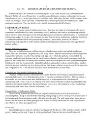
Introduction
The topography of the Earth holds endless
fascination for geologists and others who
love the natural world. Topography refers
to the hills, valleys, and other three-dimensional
landforms on the Earth's surface.
Bathymetry refers to similar features
located beneath the sea.
Landscapes are interesting because
they reflect the long-term action of erosional
forces, such as streams, glaciers, and
pounding waves at the beach, and differences
in how easily the underlying rocks
erode. By "reading" a landscape, geologists
discover rock structures hidden beneath the
soil, infer long sequences of past landscapes,
and see that the land has uplifted or
subsided. In the eyes of a geologist, a threedimensional
landscape gains the fourth
dimension of time. Archaeologists familiar
with natural landforms become adept at
spotting unnatural features, which helps
them discover sites of ancient human
activity.
As you will learn in this chapter, landscapes
are conveniently visualized with
the aid of maps and digital elevation models.
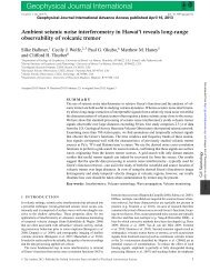
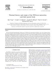
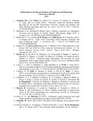
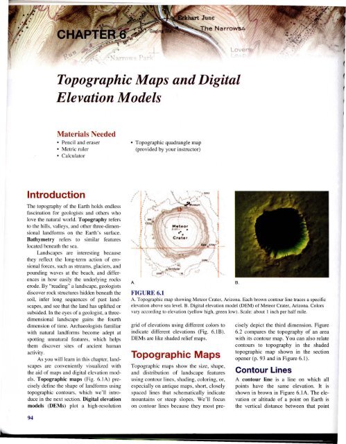
Topographic maps (Fig. 6.1A) precisely
define the shape of landforms using
topographic contours, which we'll introduce
in the next section. Digital elevation
models (DEMs) plot a high-resolution
A.
FIGURE 6.1
A. Topographic map showing Meteor Crater, Arizona. Each brown contour line traces a specific
elevation above sea level. B. Digital elevation model (DEM) of Meteor Crater, Arizona. Colors
vary according to elevation (yellow high, green low). Scale: about I inch per half mile.
grid of elevations using different colors to
indicate different elevations (Fig. 6.1B).
DEMs are like shaded relief maps.
Topographic Maps
Topographic maps show the size, shape,
and distribution of landscape features
using contour lines, shading, coloring, or,
especially on antique maps, short, closely
spaced lines that schematically indicate
mountains or steep slopes. We'll focus
on contour lines because they most pre-
B.
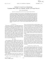
cisely depict the third dimension. Figure
6.2 compares the topography of an area
with its contour map. You can also relate
contours to topography in the shaded
topographic map shown in the section
opener (p. 93 and in Figure 6.1).
Contour Lines
A contour line is a line on which all
points have the same elevation. It is
shown in brown in Figure 6.1 A. The elevation
or altitude of a point on Earth is
the vertical distance between that point
94

Chapter 6 Topographic Maps and Digital Elevaton Models 95
Normal closed contour
has same elevation as
higher contour.
Depression contour
has same elevation
as lower contour.
200-foot
contour
Shoreline = zero-foot contour
FIGURE 6.2
The area sketched in the top diagram is shown as a topographic (contour) map in the bottom
diagram. Contour lines (brown) on the map are drawn at intervals of 20 feet, starting with 0 at
mean sea level. The fact that contours bend upstream where they cross streams allows quick
recognition of hilltops. Source: U.S. Geological Survey.
FIGURE 6.3
A normal closed contour (above left)
encircles a small hill top. If this small hill is
on the side of a larger hill, the elevation of the
closed contour is the same as the higher
contour, as shown here.
A depression contour (above right) encircles
a pit or depression in the landscape. If the
depression occurs on a slope, as shown, the
depression contour has the same elevation as
the lower contour. With a C.I. of 10 feet, the
elevation of the inner depression contour is
90 feet. The bottom of the depression is less
than 90 feet and more than 80 feet (because
there is no 80-foot contour).
and sea level, which by definition has an
elevation of zero. Figure 6.2 shows an
area along a sea coast, with the sea at its
average elevation of zero feet. Because
the edge of the shore is everywhere at an
elevation of zero feet, the shoreline coincides
with the zero foot contour. If sea
level rose by 100 feet, the shoreline
would everywhere coincide with the
lOa-foot contour shown in Figure 6.2; if
it rose 200 feet, it would coincide with
the 200-foot contour.
Contour Interval
Contour lines are drawn on a map at
evenly spaced intervals of elevation. The
difference in elevation between two consecutive
contours on the same slope is
called the contour interval (C.I.). It is a
constant for a given map, unless otherwise
stated, and is usually given at the
bottom of the map.
The choice of contour interval depends
on the level of detail the topographer
wishes to show and the range of elevation,
or relief, of the mapped area.
Florida is so flat that a 5-foot contour
interval often best captures the landscape.
The Rocky Mountains, on the other hand,
show up best with lOa-foot contours. A
5-foot interval would paint a Rockies
map solid brown with over-abundant
contours'
Index Contours
As a general rule, every fifth contour
starting from sea level is an index contour.
These are drawn as heavy lines and
labeled with their elevations (Fig. 6.2).
They make it easier to read a topographic
map. Contours between index contours
are usually not labeled.
Depression Contours
Depression contours are closed contours
with hachures (Sh0l1 lines perpendicular to
the contour line) pointing toward the lower
elevations within a depression (Fig. 6.3).
They generally encircle small depressions,
but can be used for large depressions (e.g.,
Fig. 6.1).
Contour Line
Characteristics
The construction and reading of contour
maps are governed by the following characteristics
of contour lines (most of which
are illustrated in Figure 6.2):
I. Every point on the same contour line
has the same elevation.
2. A contour line always rejoins or
closes upon itself to form a loop.
This may occur outside the map
area. Thus, if you walked along a
contour, you would eventually get
back to your starting point.
3. Contour lines never merge, split, or
cross one another. However, if there
is a steep cliff, they may appear to
overlap because they are superimposed
on one another.
-- - -~ -~ -------=--...::~~---~~~...::==---~-- ---~-
-----------

96 Part III Maps and Images
4. Slopes rise or descend at right angles
to any contour line.
• Closely spaced contours indicate a
steep slope.
• Widely spaced contours indicate a
gentle slope.
• Evenly spaced contours indicate a
uniform slope.
• Unevenly spaced contours indicate
a variable or irregular slope.
5. Contours usually encircle a hilltop.
If the hill falls within the map area,
the high point will be inside the
innermost contour (however, see
discussion of depression contours).
6. Contour lines near ridge tops or
valley bottoms always occur in pairs
having the same elevation on either
side of the ridge or valley.
7. Contours always bend upstream
when they cross valleys. Because
water runs downhill, this fact allows
the rapid recognition of high and low
areas on a contour map.
8. If two adjacent contour lines have
the same elevation, a change in slope
occurs between them. For example,
adjacent contours with the same
elevation would be found on both
sides of a valley bottom or ridge top.
9. Depression contours have the same
elevations as the normal
(unhachured) contours immediately
downhill (Fig. 6.3).
Reading Elevations
Start with a labeled index contour. As you
move uphill from this contour, keep track
of the elevation by adding the value of the
contour interval for every contour crossed.
In Figure 6.4, moving from the 200' index
contour to point X crosses two contours:
200' + 20' + 20' = 240' elevation. When
hiking downhill you subtract contour
intervals.
The elevation of a point that does not
fall on a contour must be estimated. An
estimate can be made by interpolation,
assuming the slope between adjacent contours
is uniform. For example, a point onequarter
of the way between contours with
elevations of 200 and 220 feet (C.l. = 20
feet) would have an elevation of about
205 feet. However, slopes are often not
~----------200---
c.\. = 20 feet
FIGURE 6.4
Reading elevations from a contour map with a contour interval of 20 feet. The elevation of X is
240 feet, because X falls on a contour with that elevation. Point Y falls between the 240- and
260-foot contours, so its elevation must be between those values. Its horizontal position is about
three-quarters of the way between the two, so assuming a uniform slope gives an estimated
elevation of 255 feet. Point Y has a halfway elevation of 250 ± 10 feet: 250 is halfway between
240 and 260, and ± 10 indicates that Y falls between 240 (250 - J0) and 260 (250 + 10). Note
that the error term (± 10) is found by dividing the contour interval by two. What is the halfway
elevation of Z at the top of the hill? (Answer: 310 ± 10 feet)
uniform, so another approach is to give the
halfway elevation between the two contours.
A halfway elevation is the elevation
halfway between the values of adjacent
contours; thus, the elevation of a point
between contours can be stated as the
halfway elevation plus or minus one-half
the contour interval. Figure 6.4 provides
examples.
Study of Figure 6.3 shows that a normal
closed contour that lies between a
higher and a lower contour always takes
the same elevation as the higher one. A
depression contour in the same situation
always takes the same elevation as the
lower one.
Digital Elevation
Models
A digital elevation model (DEM) consists
of a high-resolution grid of points
assigned elevations and colored according
to elevation (Fig. 6.1 B). Most DEMs
are compiled from existing topographic
maps. However, radar data from the
Space Shuttle (SRTM), specially commissioned
aircraft flights, and data from
various satellites are processed to provide
higher-resolution DEMs than are otherwise
available from such government
agencies as the U.S. Geological Survey,
the Centre for Topographic Information
(Natural Resources Canada), and INEGI
in Mexico.
DEMs make it easier to visualize
landscapes, and they often highlight subtle
features that are not obvious on topographic
maps. However, unless you have
a computer handy, topographic maps are
more useful in the field because it is
easier to read accurate elevations, spot
places that are easier or more challenging
to hike over, and find such humandesigned
cultural features as roads,
buildings, dams, and political boundaries.
If you have access to Geographic Information
System (GIS) software, you can
drape (superimpose) a variety of topographic
map features over your DEM to
get the best of both worlds.
Working with Maps
We have to cover a few "necessary
evils" before we can dive into landscapes
and topographic maps. Coordinate
systems are important because they
allow us to precisely locate points on
the Earth's surface. We also must
understand the scale of a map so we can
tell how big things are. For example, the
scale of the map in Figure 6.1 A tells us
that Meteor Crater is about I ~ miles
across and not 50 miles across. Coordinate
systems and scale are not difficult
to understand once you get used to
them, but they will take some extra concentration
as you read the next few sections.
Understanding these concepts is

Chapter 6 Topographic Maps and Digital Elevaton Models 97
also important if you plan on taking a
GIS class in the future.
Map Coordinates
and Land
Subdivision
Coordinate systems provide a permanent
way of describing locations. For example,
older descriptions of mineral or fossil sites
commonly refer to landmarks. Unfortunately,
some of these old sites are now lost
because road intersections, houses, small
bridges, old trees, and railway lines have
since been moved or removed due to
ongoing development. A coordinate system
allows a state to efficiently and pennanently
keep track of the locations of abandoned
oil wells, toxic waste sites, sealed
mine shafts, and places hosting endangered
plants or breeding pairs. It allows
geologists to describe important rock
localities, and it allows hikers to precisely
locate trailheads, remote camp sites, and
other places worth remembering.
Latitude-Longitude
System
The most well-known global coordinate
system is based on east-west lines called
lines of latitude and north-south lines
called lines of longitude.
Latitude measures distance north or
south of the equator. The lines of latitude,
also called parallels, form a series of parallel
circles running east-west (horizontally)
around the globe. The equator represents
the 0° latitude line. Other parallels
are set at angular intervals measured
north or south of the equator, as shown in
Figure 6.5A. A latitude line 40° north of
the equator is termed 40° N. The geographic
poles are at 90° and 90° S.
Longitude measures distance east or
west of the Prime Meridian. Lines of longitude,
also termed meridians, form a
series of circles running north-south (vertically)
and intersecting at the geographic
poles. The Prime Meridian is the northsouth
line passing through the Royal
Observatory in Greenwich, England; it is
defined as 0° longitude. The other meridians
are set at angular intervals east or
west of the Prime Meridian, as shown in
A.
Equator

860
(
,J r
1--' _ \
J C'\ i21"...
\ )/1:925 .'V \!.Y
U ( r \) _ _ ~ 936
B II N-r/ eRE E K
/ ~ J
\ I t././ -' -'
T 114 N
T 113 N
----''----'-~
~"__'___t'_----'L----'----'-L----'--'---~-JU..L-----'--LL'---'~-----''-'--L.~-=='''--~., -44°37'30"
• INTERIOR-GEOLOGICAL SURVEY RESTON V1AGtN1A-1982 93037'30"
'50 00om E
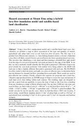
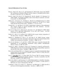
FIGURE 6.6
This corner of a quadrangle map shows the latitLIde and longitude of its southern and eastern boundaries, UTM grid coordinates, and township and
range designations (red). The UTM grid is shown with thin black lines. Along the side, 49 45 is shorthand for 4,945,000 mN and 49 43 000 mN for
4,943,000 mN. Similarly. along the bottom, 4 48 is shorthand for 448,000 mE and 4 50 000 mE for 450,000 mE. On a full-sized map, the zone number
is found in the lower left corner in the fine print. This map falls within zone 15.
UTM example: A given house (small black square) falls within a 1000-m square defined by grid lines 4,942,000 mN (south side), 4,943,000 mN
(north), 449,000 mE (west), and 450,000 mE (east). To determine its coordinates, measure in millimeters the distance from the 4,942,000 mN line to
the house and then the total distance to the 4,943,000 mN line. The house is located 39 mm out of a total 42 mm between grid lines. [n percent,
39/42 = 0.93 or 93%. Since the grid distance represents 1000 m, the house is located 0.93 X 1000 = 930 m above the southern line, or at
4,942,930 mN. Similarly, the house is located 20 mm/42 mm or 48% of the way east of the 449,000 mE line. This equals 449,480 mE. The location
of the house, to within a 10-m square, is formally given as: 4,942.930 mN; 449,480 mE; Zone 15; northern hemisphere.
98

Chapter 6 Topographic Maps and Digital Elevaton Models 99
96" 95" 94" 93" 92" 91" 90" W
48°N -rt-+--++--+---4+--+--t-r-~
5,400,000 mN
5,300,000 mN
-+-+-+--+1--+--++--+-+-+ 5,200,000 mN
+-+--+---++--1--++--+-+-+ 5,100,000 mN
lambert Equal Area Projection
A.
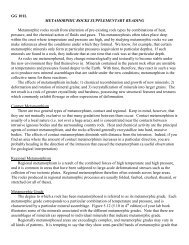
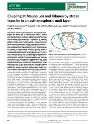
FIGURE 6.7
A. UTM-grid zones in North America. Each zone is 6° of latitude wide. The
zones are numbered counting west to east from the International Date Line.
At the middle of each zone is the central meridian used to set up the eastwest
1000-meter UTM grid lines.
B. Example showing two parts of the UTM grid for zone 15 (black lines).
The lines of latitude and longitude are in red. The grid system counts
meters north of the equator and east or west of the central meridian, which
is arbitrarily set to 500,000 meters. The lines on the two grids are parallel
near the equator but not at higher latitudes because most latitude and
longitude lines are projected as curves, whereas UTM lines are drawn as
straight lines on this projection. The point in the shaded area is located in
Figure 6.6.
+-+-+--I-I--+---+t----+---+--+ 5,000,000 mN
44°N -~:t:t=:=+t==t:=:tt:=~:::t:4,900,000 mN
! I
II
w E
o
,8
I~
w Eo
.........~r'--, ;-,
I I ' ! ,
w J.J ~ 'w
E E E E
8 8 § g
8 8 8' g\
1.0 (0 I'-- co,
10
o
/8 "
+-+--++---++--+---j-+---1-+-+-+- 400,000 mN
-+-+---1-j---+I---+---++--H--+--+- 300,000 mN
2°N --=l:::t=ti=:tt:=::j::=~=t:t=::j:::t 200,000 mN
-+-+---1-+--++---+---++--H--+--+- 100,000 mN
91"
90" W
Because the Earth is round, even small
areas (like the shaded one in Fig. 6.5B)
represent curved surfaces that must be
shown on flat maps. This requires a projection
of the three-dimensional curved surfaces
onto a two-dimensional sheet of
paper. Many ways have been developed to
accomplish this-names such as "Mercator
projection" or "polyconic projection" may
be familiar to you-but all unavoidably
result in some sort of distortion and create
certain difficulties.
Universal Transverse
Mercator (UTM)
System
A second widely used global coordinate
grid is the UTM system. Its set-up may
seem somewhat complex, but the UTM
system produces a handy grid of I-km
squares on many maps. This makes it
easy to determine accurate grid coordinates
from paper maps and to determine
distances between points. Most global
positioning system (GPS) units allow you
to switch between latitude-longitude and
UTM coordinates.
The UTM system divides the 360°
range of longitude into 60 north-south
zones, each 6° wide. Figure 6.7A shows
these zonc:s in North America. The
zones are numbered from west to east,
beginning at the International Date
Line. The zone number is given in fine
print in the lower left corner of USGS
quadrangle maps. Each zone is divided
into a grid with its origin at the intersection
of the equator and its own
central meridian, as shown for zone IS
in Figure 6.7B (e.g., 93° W is the central
meridian between 90° to 96°). A
metric grid, with lines intersecting at
right angles, is developed from this origin
on a transverse-Mercator-type map
projection. Lines running east-west
count the number of meters from the
equator. North-south lines measure the
number of meters from their zone's
central meridian, which is arbitrarily set
to a value of 500,000 m to avoid coordinates
with negative numbers (study
Fig.6.7B).
Features are located by their UTM
coordinates. UTM coordinates are given
by distinctive numbers (e.g., 49 44°00,
49 45) along the margins of USGS maps
(Fig. 6.6). The numbers give the distance
in meters from the zone origin. In Figure
6.6, for example, 49 43°00 mN describes an
east-west line 4,943,000 m (4943 km)
north of the equator. The east-west line
I km (1000 m) to the north is 49 44°00 mN.
The larger "44" makes it easier to count
the I-km increments. The complete UTM
coordinate is given as: north-south coordinate
(northings), east-west coordinate
(eastings), zone number, and hemisphere
(north or south). Because some give the
east-west coordinates first and the northsouth
coordinates second, it is essential to
label your UTM coordinate numbers with
"mN" (meters north) and "mE" (meters
east). Figure 6.6 gives a worked example
determining UTM coordinates.

100 Part III Maps and Images
A.
R4E
B.
Correction
line
}Tier
3S (T3S)
\Correction
line
SE)4, NW)4, Sec. 16, T3S, R4E
NW)4
NW)4
FIGURE 6.8
U.S. Public Land Survey subdivision, illustrated by successively smaller areas. A. Example of a
baseline and principal meridian in the western United States. The area to which they apply is
shaded. B. From a starting point at the intersection of a principal meridian and a baseline, 6-milewide
tier and range bands subdivide land into 36-square-mile townships. C. Townships are
subdivided into 36 I-square-mile sections. D. Sections can be divided into halves, quarters,
eighths, or other fractions.
R5E
24 T2S
~ G 29
31 32 33 34 35 36
3 ?- /( 6 5 4 3 2 1 6 lE
V 12 7 8 9 10 11 12 7
,
-fa 18 17 16 15 14 13 18
T3S
R4E
~ 24 19 20 21 I~~ 24 19 A
C.
Wyoming
R3E
Base
Colorado
South
Dakota
Nebraska
line
Kansas
T3S
1""- 25 30 29 28 27 26 § ;::::-..
I~ 31 32 33 34 35 36 31 tt-
-?..>
:q 6 5 ~ 3 2 1 F
--¥ H 0 T4S
u.s. Public Land
Survey System
The U.S. Public Land Survey System was
designed to efficiently describe areas of
land in most states outside of the original
13 colonies. This system, commonly called
the Township-Range system, was started in
1785, when the old Northwest Tenitory
(Lake Superior region) was opened to
homesteading. It has been widely used for
ordinary and legal land descriptions in the
western two-thirds of the United States
ever since. The method subdivides land
into 6- X 6-mile squares called townships;
these are further subdivided into 1- X
I-mile squares called sections.
D.
E~
The starting point for subdivision is
the intersection of selected latitude and
longitude lines. The starting latitude is the
baseline, and the starting longitude is the
principal meridian. Baselines and principal
meridians are established for a number
of areas in the United States; an
example is shown in Figure 6.8A. Lines
drawn 6 miles apart and parallel to the
baseline form east-west rows called tiers.
North-south lines parallel to the principal
meridian and 6 miles apart form northsouth
columns called ranges (Fig. 6.8B).
The squares formed by the intersection of
tiers and ranges are called townships.
Each township is approximately 6 miles
square and has an area of about 36 square
miles. Political townships, usually named
after the largest town within the area at
the time they were designated (for example,
Baraboo Township, Wisconsin), may
or may not coincide with Public Land
Survey townships.
Tiers and ranges are numbered by reference
to the baseline and principal meridian
(Fig. 6.8B). The first tier north of the
baseline is Tier 1 North (abbreviated TIN);
one in the fifth tier to the north is T5N, and
so forth. Ranges are numbered to the east
of the principal meridian (for example,
R5E) and to the west (R2W). A Public
Land Survey township (like the shaded one
in Fig. 6.8B) is located using tier-range
coordinates: T3S, R4E. NOTE: Tier is
always written first, range second.
Because lines of longitude (meridians)
converge toward the poles, it is
impossible to maintain squares that are
6 miles on a side. Thus, a correction is
made at every fourth tier line (labeled correction
line on Fig. 6.8B), and new range
lines 6 miles apart are established. The
cOlTection restores townships immediately
north of the line to their proper size.
Each 6-mile-square township is subdivided
into thirty-six, 1- X I-mile squares,
called sections, which are numbered in a
specific sequence (Fig. 6.8C). Each section
consists of 640 acres. A section is subdivided
into halves, quarters, eighths, sixteenths,
and so on (Fig. 6.8D). A sixteenth
of a section is 40 acres.
Points are located according to the
smallest subdivision required. In Figure
6.8D, the star is located, to the nearest
40 acres, in the SE )4, NW )4, Sec. 16,
T3S, R4E. Locations are always written
from the smallest unit to the largest, and
tier is written before range.
Section numbers and tier and range
values are written in red on USGS topographic
maps (see Fig. 6.6).
Map Scale
The scale of a map is essential because it
tells the user the size of the area represented
and the distance between various
points. Three types of scales are in common
use: ratio, graphic, and verbal scales.
A ratio or fractional scale, shown at
the bottom of Figure 6.9, is the ratio
between a distance on a map and the
actual distance on the ground. The ratio

U.S. Public Land Survey
Range coordinate
r
Intermediate
longitude
(in minutes and seconds)
rUTM coordinate
(without zeros;
kilometers east)
MT. SHASTA QUADRANGLE
CAUFORNIA -- SISKIYOU CO.
7.5 MINUTE SERIES (TOPOGRAPHIC)
U.S. Public
Land Survey
tiercoo~
U.S. Public
Land Survey ~
section number/' -
StatePla~
coordin~t~" ~
number (not
discussed)
Map data,
including UTM
......-.s-"""'-......'_
zone and the '=.~~~":.__ _ \V _
North :2-=::?:::'-:7-_ 1~ 11.5._. 8 =~----
American _....:::-~.::.:.:=..-=.-_"';';' 13 -----
Datum to use ~::.:::=E:.:::r=:-: ...L~~==:::;;:-""""t__;::=:;::'~=~~::::':'::~~=-_;:::±:;:=7"""rrl"'T'J"T'J:~~ .__ 0 ::;"---- ---
in your GPS _=~:'::J::.:""':__~. Contour • :::::..-- :::-'::~:-""a ~ ==-
FIGUR~e:~;er.\. ~...:=;:...-::.::..-:.:==;=.- ,',:-. ";'':: ~ interval • !~~~-::=C MT. S~A, CA )
"'--J Magnetic declination Names of ,--..- t
Reduced copy of the Mt. Shasta, California, 7'/,- (MN) adjoining---... '-----t--+---I~=--
d I r- 6CllyofMt.Sh-.
minute quadrangle, with principal map features qua rang es ~~ Name of quadrangle
highlighted and magnified. """'""""". and year of publication
101Xll

102 Part III Maps and Images
scale on Figure 6.9 is I:24,000 (or
1124,000), which means that one unit (for
example, an inch) on the map equals
24,000 of the same units on the ground.
A graphic scale usually consists of a
scale bar subdivided into divisions corresponding
to a mile or kilometer (see Fig.
6.9). One mile or kilometer segment on
the scale bar is commonly subdivided to
allow more precise measurements of distance.
The subdivided units are commonly
placed to the left of zero on a scale bar, as
in Figure 6.9. A graphic scale is helpful
because it is readily visualized and stays
in true proportion if the map is enlarged or
reduced. It also provides a convenient way
of measuring distances between points on
a map: lay a strip of paper between the
points and make pencil marks next to
each point. Then lay the paper along the
graphic scale at the bottom of the map and
determine the distance.
A verbal scale is commonly used to
discuss maps but is rarely written on
them. People usually say, "I inch equals
I mile," which means, "I inch on the map
represents, or is proportional to, 1 mile
on the ground." Because I mile equals
63,360 inches, a common fractional scale
of 1:62,500 on older maps corresponds
closely to the verbal scale "I inch to
I mile." Many U.S. maps, and essentially
all foreign maps, use metric scales, making
common fractional scales easily convertible
to verbal scales: scales of
I:50,000, I: 100000, and I:250,000 correspond
to I centimeter equaling 0.5, 1.0,
and 2.5 kilometers, respectively.
4° quadrangle maps are drawn at a
fractional scale of I: I,000,000; 2° quadrangles
at I:500,000; I° at I:250,000; 15' at
I:62,500 or I:50,000; and 7'.1.' at 1:24,000
or 1:25,000. Both graphic and fractional
scales are shown at the bottom center of the
map (see Fig. 6.9).
These different scales are used to
show larger or smaller areas of the Earth's
surface on conveniently sized maps. For
example, it may be possible to show a
small city on a map where I inch on the
map represents 12,000 inches (1000 ft) on
the ground. This map would have a scale
of I: 12,000. However, to show a midsized
state, such as Indiana, on a map of
similar size, the scale would have to be
much smaller, say I inch on the map to
500,000 inches (approximately 8 miles) on
the ground. In general, the larger the area
shown, the smaller the scale of the map
(smaller because the fraction 1!500,000 is
a smaller number than 1/12,000).
Converting Among
Scales
Verbal to fractional scale
conversion:
I. Convert map and ground distances
to the same units.
2. Write the verbal scale as the fraction:
I. Convert both map and ground distances
to the same units, inches:
5000 X 12" = 60,000". The verbal
scale is now 2.5 inches on the map
represents 60,000 inches on the
ground.
2. Write the verbal scale as the fraction:
2.5" (distance on map)
60,000" (distance on ground)
3. Divide the numerator and denominator
by the value of the numerator:
2.5"/2.5"
60,000"/2.5"
Distance on map
Distance on ground
3. Divide both numerator and denominator
by the value of the numerator:
Distance 0/1 map/distance on map
Distance on ground/distance on map
Example: Convert the following verbal
scale to a fractional scale: 2.5 inches on
the map represents 5000 feet on the
ground.
I
24,000 or 1:24,000
Fractional to verbal scale
conversion:
I. Select convenient map and ground
units to relate to each other (for
example, inches and miles or centimeters
and kilometers).
2. Express fractional scale using the
map units (inches or centimeters).
3. Convert the denominator to the
ground units (miles or kilometers).
4. Express verbally as "I inch [or
I centimeter] equals X miles [or
kilometers]."
Example: Convert a fractional scale of
I:62,500 to a verbal scale of I map inch
equals X miles on the ground.
I. Units to be related are inches and
miles.
2. 1:62,500 = 1"/62,500"
3. Convert 62,500" into miles by dividing
by the number of inches in
I mile. One mile = 5280 feet and
1 foot = 12 inches. So, 1 mi =
5280' X 12" = 63,360". Working
out the division:
62,500 inches .
63 360 ' I . = 0.986111/
, mc 1es per 1111
4. Expressed verbally, I inch on the
map equals 0.986 mile on the
ground.
Magnetic
Declination
Maps are usually drawn with north at
the top. North on a map refers to true
geographic north. At most places on
Earth, however, a compass needle does
not point toward the geographic north
pole but toward the magnetic north pole.
The magnetic north pole is in the
Canadian Arctic, but its exact position
changes. For example, in 1955, it was
located north of Prince of Wales Island
near latitude 74° N, longitude 100° W;
its last measured location in 200 I put it
in the Canadian Arctic Ocean (81.3° N,
110.3° W) headed northwest toward
Siberia at 40 km/year.
The angular distance between true
north and magnetic north is the magnetic
declination. Because the location
of the magnetic pole changes, the magnetic
declination generally varies with
time. If you are navigating or doing geologic
research using a compass, you
must adjust the declination of the compass
for local conditions. Without
adjustment, compass errors in excess of
10° to 20° are possible along the west
and east coasts of North America! The
magnetic declination is shown at the
bottom of most USGS maps by two
arrows (see Fig. 6.9). One points to true
north (commonly marked with a star, or
T.N.) and one points toward magnetic
north (commonly marked M.N.). The

Chapter 6 Topographic Maps and Digital Elevaton Models 103
angular separation between them (the
magnetic declination) also is given.
When stating the magnetic declination
of a map, it is always necessary to indicate
whether the arrow pointing to the
magnetic pole is east or west of the geographic
pole. If it is east, the declination
is stated as so many degrees east, for
example, 212° E. Most maps also have
an arrow pointing toward G.N., the
location of the grid north direction for
the Universal Transverse Mercator
(UTM) grid system (see Fig. 6.9).
Symbols
Standardized symbols and colors are used
on government maps to designate various
features. On USGS maps, cultural features
(those made by people) are generally
drawn in black; forests or woods are
shown in green (they are not always represented);
blue is used for bodies of
water; brown shows elevation (contours),
some mining operations, and beaches or
sand areas; and red is used for the better
roads and some land subdivision lines.
See Figure 6.10 for symbols and Figure
6.9 for some examples. Note that when
USGS topographic maps are revised, any
new features (e.g., roads, suburbs, strip
mines) that appear in an area are colored
purple. Symbols for Canadian government
maps are shown on the backs of the
maps. Mexican map symbols are generally
on the front.
Working with
Topographic Maps
Now that you understand contours, coordinate
systems, and scale, we are ready to
cover some ways of working with topographic
maps. We'll start with the basics
of how topographic maps are produced.
Making Topographic
Maps
Making a topographic map requires accurate
points of elevation in the map
area. A bench mark is a point whose
elevation and location have been precisely
determined by government surveyors;
its location is marked by a small
brass plate. Bench marks are designated
on maps by the symbol B.M. (Fig. 6.9).
Spot elevations are somewhat lessprecisely
determined elevations used in
the construction of topographic maps.
They are shown at many section corners,
bridges, road intersections, hilltops,
and the like and may be marked
with an "x" (examine Fig. 6.9). Bench
marks and spot elevations are used in
conjunction with aerial photographs to
construct topographic maps. Two aerial
photos, taken from different points but
overlapping the same area, provide a
three-dimensional view of the land surface
when viewed through a stereoscopic
viewer. By orienting the photos properly,
two beams of light from different
sources can be focused at any elevation.
If the superimposed beams are moved
around a hill, for example, they will
trace a line at a precise elevation. The
numerical value of this elevation can
be determined from known elevations
within the area (e.g., bench marks). Aerial
photographs are discussed further in
Chapter 7.
If you are a landscaper or an architect,
for example, you may want to make
your own detailed topographic map of an
area. You can start by tracing any important
features (drainages, coastlines,
buildings, etc.) from an air photo
obtained from the USGS or from your
state. Then, starting from the lowest spot
on the property, take a series of hikes
uphill with a 5-foot staff and a spirit
(bubble) level that allows you to site
horizontal lines from the top of your
staff. These allow you to plot successive
elevation increments of 5' on your map
(Fig. 6.l1A). Now add the contours to
reflect the landscape by following these
steps:
I. Select a contour interval that will
show the level of detail you need.
Too many contours can be confusing.
2. If your staff was a convenient length
(e.g., 5 feet), simply connect those
points that correspond to multiples
of the contour interval. If the c.I. is
20 feet, you would connect dots
marking 20, 40, 60, etc., feet.
3. Draw fairly smooth, fairly parallel
contours, but be sure to bend them
upstream when crossing drainages
and gullies (Fig. 6.l1B). Adding
extra wiggles implies you know
more than you do. Draw the lines to
the edge of the map. Label each
contour or index contour with its
elevation.
Topographic Profiles
A topographic profile shows the shape
of the land surface as it would appear in a
cross section; it is like a side view. Topographic
profiles portray the shape of the
land surface along a particular line of profile.
They are useful for many practical
purposes, such as planning roads, railroads,
pipelines, hiking trails, and the
like, or for estimating the volume of
material that will need to be excavated or
filled during road construction. Profiles
are most easily made along straight lines,
but they can also follow curved paths,
such as a road or a stream.
A topographic profile is made from a
contour map using the following procedure
(Fig. 6.12):
l. Select the line or path along which
the profile is to be made, such as line
X-Y in Figure 6.l2A.
2. Record the elevations along the line
as shown in Figure 6.12B. To do this,
lay the straight edge of some scratch
paper along the line of profile. Mark
on the paper the ends of the profile
line and the exact place where each
contour line meets the edge of the
paper. Label each mark on the paper
with the elevation of the corresponding
contour. Also mark the positions
of any streams that cross the line of
profile, because they will be low
points on the profile.
3. Set up the graph on which the profile
will be drawn (Fig. 6.l2C). First note
the differences in elevation between
the highest and lowest points along the
line of profile; this will determine the
range of elevations on your profile.
Label the vertical axis with a range of
elevations that extends beyond the
profiJe elevations and conveniently
allows each contour to be graphed. In
Figure 6.l2C, the profile elevations
range between 820 and 940 feet and
are spanned by a vertical axis of 700
to 1000 feet. Horizontal lines on the
vel1ical axis are 20 feet apart, which
matches the contour intervaJ and
makes graphing simple. CommonJy,

Topographic Map Symbols
BOUNDARIES
RAILROADS AND RELATED FEATURES
COASTAL FEATURES
National. .
......_-- Standard gauge single track; station..
Foreshore flat (shallow sediment).
State or territorial
_ Standard gauge multiple track .
Rock or coral reef .
County or equivalent. --- Abandoned .
Rock bare or awash ..
Civil township or equivalent.
Incorporated-eity or equivalent. .
.... . 1-_, _
. .r- - - - -
Under construction
Narrow gauge single track .
.
Group of rocks bare or awash.
Exposed wreck......................•..
Park, reservation, or monument. ..
.I-- . _ Narrow gauge multiple track .
Depth curve; sounding .
Small park .
Railroad in street. .
Breakwater, pier, jetty, or wharf.
Juxtaposition........................•.
Seawall ..
LAND SURVEY SYSTEMS
Roundhouse and turntable .
U.S. Public Land Survey System:
Township or range line.
TRANSMISSION LINES AND PIPELINES
BATHYMETRIC FEATURES
Area exposed at mean low tide; sounding datum ._...../.
Location doubtful. ... f- _ _ _ Power transmission line: pole; tower..
Channel .
Section line
f-----j Telephone or telegraph line.
Offshore oil or gas: well; platform . o •
Location doubtful. --- Above-ground oil or gas pipeline.
.~__~ Sunken rock.
Found section corner; found closing corner I- ~ ~_ Underground oil or gas pipeline .
Witness corner; meander corner ~c1+ _ ~
RIVERS, LAKES, AND CANALS
I MC,
CONTOURS
Intermittent stream . . ....---. .
Other land surveys:
Topographic:
Intermittent river .
..... - ..::::::
Township or range line.
Section line.
Intermediate .
Disappearing stream.
.. .. ---<
Land grant or mining claim; monument.. ..... +_ _ to
Index .
Perennial stream.
Fence line ..
Supplementary .
Perennial river .
Depression ..
Small falls; small rapids .
ROADS AND RELATED FEATURES
Cut; fill ..
I-."~"";,.j Large falls; large rapids .
Primary highway..
f---~ Bathymetric:
Secondary highway..
Intermediate.
Masonry dam .
Light duty road.
Index.
Unimproved road.
Primary..
Dam with lock.
Trail. .
Index Primary .
Dual highway.
Supplementary.
Dual highway with median strip .
Dam carrying road.
Road under construction . ~_~ MINES AND CAVES
Underpass; overpass.. .~ Quarry or open pit mine .
Intermittent lake or pond , .
Bridge . I-__~ Gravel, sand.. clay, or borrow pit. .
Dry lake ..
Drawbridge.
I-__~ Mine tunnel or cave entrance.
Narrow wash.
Tunnel.
. 1-0"""'- Prospect; mine shaft. .
Wide wash .
','
Mine dump ..
Canal, flume, or aqueduct with lock .
BUILDINGS AND RELATED FEATURES
Dwelling or place of employment: small; large.. • _
Tailings .
Elevated aqueduct, flume, or conduit.
Aqueduct tunnel.
School; church. •• SURFACE FEATURES
Barn, warehouse, etc.: small; large. 0 ~ Levee
Water well; spring or seep .
House omission tint.
Sand or mud area, dunes, or shifting sand.
GLACIERS AND PERMANENT SNOWFIELDS
Racetrack .
Intricate surface area.
. >'-

Chapter 6 Topographic Maps and Digital Elevaton Models 105
x
15
A.
x
x15 25
x26
x20 2~
/
23 x
x 20
x 15 x
15 x / 20
x x 10 x
15 10 x
/ 15
x x 5 x
10 5 10
x
x 5
5
A. B.
FIGURE 6.11
How to make a contour map: A. Elevations from numerous transects across the area are added to
a sketch map. B. Smooth contour lines connect the dots at the elevations corresponding to the
contour interval. Lines are smooth except where they cross drainages.
I i I i I I I I I
I
i i I i i i I
X~ 0 0 0 0 0 0 0 0 0 0 00
c;o co 0 0 co c;o
E 't c;o co 0C\j
co co co ~
~Y
0) 0) co co Cll co co co 0)0)
~
1000 ,---;.--+--+-+--+---;----;-----+---">--+-;--+---;..->--.---+,-----------,1000
--
900 1--+-+---+:-./---="'="-:::__ :---+------'f------t----...;--+--7:/---,1:"--/---+----1900
:./ :/
:/ --:/
c.
800f--------------------------jf---I800
x
y
y
4.
as here, the vertical and horizontal
scales are different. In Figure 6.l2C,
the horizontal scale is about I" equals
800' (1:9600) whereas the vertical
scale is 1" equals 160' (1:1920). If the
scales were the same, the profile
would look flat. Use of an expanded
vertical scale highlights (exaggerates)
topographic variations.
Transfer each mark made along the
profile to the appropriate place on
the graph paper by aligning the
paper with your graph (Fig. 6.12C).
Mark the ends of the profile on the
graph paper. Mark the contour and
stream points on the graph at their
appropriate elevations. This is done
by going straight up from the mark
on the paper (or, as illustrated here,
down from the top of the graph
paper with the marks made directly
on it) to the horizontal line representing
the same elevation; make a
small dot on the paper at this point.
5. Connect the points on the graph
paper with a smooth line representing
the topography (Fig. 6.12C).
When crossing a valley or a hilltop,
there will be adjacent marks with the
same elevation. Instead of connecting
them with a straight line, draw
your profile line so it goes up over a
hilltop or down into a valley. In the
case of a stream valley, the low point
in the valley will be where the
stream crosses the line of profile.
Vertical Exaggeration
of Topographic Profiles
Profiles are commonly drawn with a vertical
scale that is larger than the horizontal
scale. This vertical exaggeration reveals
topographic features that otherwise might
not show up on the profile. The amount of
vertical exaggeration is determined by the
ratio of the horizontal map scale (for
FIGURE 6.12
Construction of a topographic profile.
A. Choose a line of profile (X-Y). B. Mark
intersections of contours and the stream, and
note elevations on paper laid along the profile
line. C. Choose a vertical scale, and transfer
the points from the previous step to the
appropriate elevations. Connect the points
with a smooth line to complete the profile.
--~----- - - ---- . ----------

106 Part III Maps and Images

I Hands-On
Applications
You are probably already familiar with maps used to display roads and political boundaries. The handson
exercises that follow develop the basic skills needed to use and interpret the information-rich topographic
maps. As you will see throughout this lab manual, such maps are essential for recognizing and
understanding the character, origin, and even future of many landscapes. You will also see how geological
data, when plotted on maps, can clearly present a picture that is difficult to see without a great
deal of field work. Learn well the skills in this chapter, for they will serve you over and over again
throughout this class. You will also draw upon these skills if you choose a career dealing with any
aspect of the Earth's surface (e.g., in geology, environmental remediation and planning, land use planning,
archaeology, biodiversity and ecologic assessment, resources management, parks and recreation,
civil engineering, etc.).
Objectives
If you are assigned all the prob- 6. Number the sections of a direction of stream flow, and
lems, you should be able to: township if they are not already locations of hills and valleys.
numbered on the map.
1. Define latitude and
13. Determine the contour interval
longitude. 7. Determine the scale of a map and of a map.
use it to measure distances.
2. Describe the boundaries of a
14. Make a topographic map using
quadrangle map in terms of 8. Convert among verbal, fractional, points of elevation to draw
latitude and longitude, and and graphic scales. contour lines.
locate a point on a map using 9. Give the magnetic declination of IS. Construct a topographic profile
these coordinates. a map (assuming it is printed on and determine its vertical
3. Locate a point using the the map) and explain what it exaggeration.
Universal Transverse means. 16. Detennine the gradient of a
Mercator (UTM) system. 10. Determine what the various stream using a topographic map.
4. Locate or describe a parcel of symbols used on a map mean
land using the U.S. Public
(symbols for streams, roads,
Land Survey System, and
houses, etc.).
give its area in acres.
11. Use a contour map to determine
S. Give the dimensions and area elevation, height, and relief.
of a section and township (in 12. Use the characteristics of contours
miles and square miles).
to determine steepness of slope,
Problems
1. The basics of USGS topographic maps: Examine the map provided by your instructor to answer the following questions. Tables
to convert between different units are found inside the back cover. Show any calculations you make.
a. What is the name of the quadrangle and in what year was it last published or revised?
b. As frequently happens, you become interested in a feature that goes off the map. What are the names of the quadrangles to
the east and southeast?
107
- - ----~--------- ~-

108 Part III Maps and Images
c. What is the northern boundary latitude?
Southern boundary latitude?
Western boundary longitude?
Eastern boundary longitude?
Subtract these latitude and longitude numbers to get the size of the quadrangle in units of degrees, minutes, and seconds.
d. What is the fractional scale of the map?
Determine the approximate verbal scale: I inch =
miles. As always, show your calculations.
An environmental restoration project requires that you enlarge part of the map to a scale of 1 inch to 1000 feet. Calculate
the factor by which it needs to be enlarged.
What would the enlargement factor be if you needed a scale of 1 em to 100 m? Hint: Start with the fractional scale.
e. What is the contour interval?
f. What is the highest elevation within the area designated by your instructor?
What is the lowest elevation in that area?
What is the relief of the designated area?
g. What is the height (not the elevation) of the location designated by your instructor?
h. Give the elevation of the location designated by your instructor.
I. Determine to the nearest minute the approximate latitude and longitude of the designated feature.
j. Determine to the nearest 100 m the full UTM coordinates of the designated feature.
k. If the map is subdivided by the Township-Range method, locate the feature designated by your instructor to the nearest Y,6th
of a section.
I. What is the approximate size of the area designated by your instructor (in acres, if subdivided by the Township-Range
method, in square meters if the UTM method is preferred)?
m. Use the graphic scale to determine the distance in miles and kilometers between the features designated by your instructor.
n. In what direction does the water flow in the stream designated by your instructor?
o. What is the magnetic declination (in degrees) indicated on the map? In which year was this value measured?

Chapter 6 Topographic Maps and Digital Elevaton Models 109
2. Analyze a landscape: Let's say that you're a developer with a big project in mind for an area near Averill, Vermont
(Fig. 6.15). You first need to study a topographic map to understand the landscape. Show any calculations you make for the
following questions. Conversion factors are listed inside the back cover.
a. Determine the following basic facts about the map:
Interval between index contours:
Contour interval (units in feet):
Fractional scale (Hint: Use the UTM grid and metric units.):
Verbal scale (I inch =
miles):
Approximate height and width of the map. (Hint: Use the UTM grid as a bar scale.)
Approximate height and width of the map in miles (Hint: Use the verbal scale and a ruler.):
By what factor was this map enlarged or reduced from its original 1:24,000 scale?
b. To get a feel for the landscape, find the three most prominent mountains rising above 2200 feet. List their elevations starting
with the mountain near the top of the map and going clockwise. The "T" following the bench mark elevations means they
were determined from air photo measurements, which have errors of a few feet relative to the more accurate method of
surveying.
c. Determine which way the streams flow by looking at how the contours are deflected as they cross them. Draw arrows
showing the flow directions of the streams flowing into or out of the ponds and lake.
Which ponds or lakes flow into each other? (You can double-check your inferences by noting water level [WL] elevations.)
Use the stream drainages to help you find the lowest elevation on the map. What is this elevation?
What is the total relief of the map area?
Let's say that you plan to hike up Brousseau Mountain from a canoe beached on Little Averill Pond. What is the height of
Brousseau Mountain relative to this starting point?
d. At the top of Brousseau Mountain you plan on checking your hand-held Global Positioning System (GPS) unit to be sure it
works. Note that UGSG maps show latitude and longitude divisions no finer than 2' 30" (see left map margin), so you have
to switch your GPS unit to UTM coordinates. Use the map to determine the UTM grid coordinates you expect to see when
you reach the peak of the mountain (marked with an elevation on the map).
e. Because your development plans include golf courses, a water park, factory outlet shopping, and extreme paintball, you need
quite a bit of land around the Averill ponds. Do the little black dots on the map represent anything relevant to your
development plans? Explain.

(
FIGURE 6.15
Portion of the Averill, Vermont, 7 ~-minute quadrangle
map for use in Problem 2. Canada is just a few kIn north
of the map area. Scale and contour interval are determined
as part of Problem 2.
110

Chapter 6 Topographic Maps and Digital Elevaton Models III
o -------------.-----------------------------..------- .. --------..--------.---------------------------.----------------------------.-----------------.------------------------------------.--------------------------.----------------.-------------------------­
55-----------------------------------------------------.-.--...---- ..-.....----- ..--- ....-------------------------------------------­
C\J -------------.--••••••••-•• -••• -.-.-.---------.-------••• --------.-------•• -------- •• -------•• -------- •• --------.-------- •• --------.-------- •• ------ •• ------- •• --------.-- ----- •• --------.-------•• --------.--------.--------.-------•••• -------.-------
o ---- --- ------.--------.-.-- - --.--.- -.---- - ----- -..---........... ----.- - -------.--- - ---- .
8- ---.-------------..--.------ -..------------------------------------------------------------------------------------------------
C\J ••••••••••••••••••-•••••••••••••••••••••••••••••••••••••••••••••••••••••••-.---.---.--••••••••-•• -••• ----------------.--•• ----. --------.--------.-.------.-------- •• ------- •• --- •• -••• --------. --------•• -- •••••••• -•••••• ----------------••••••••-.-••• --
o
55 .......---------------------------------------------------'
~A
A'
FIGURE 6.16
Blank graph for constructing the topographic profile of Problem 2. The vertical axis marks feet above sea level.
f. Being a developer of taste and refinement, you'd like to put your name in 20-foot-tall neon letters on the top of Brousseau
Mountain. But will your guests be able to see your name from the lodge dining area to be located at point X on the map? To
find out, construct a topographic profile along the line A-A' on Figure 6.15. To save time, use just the index contours except
when marking the elevations of hilltops and valley bottoms. Draw your profile on the graph provided (Fig. 6.16). Label
"Brousseau Mountain," "Great Averill Pond," and "Black Brook" on your profile. Draw a 20-foot letter on Brousseu
Mountain and see if there is a direct line of sight from point X (the future dining room) to the letter.
Will the guests be able to see your name in lights?
What is the vertical exaggeration on the profile you drew? Show your work.
3. Comparing a contour map with a DEM: Figures 6. J7 and 6.18 show the area around Mono Lake, CA. Use these figures to
answer the questions that follow.
a. Determine some basic facts about the map (Fig. 6.17):
The contour interval is 200 feet. In low-relief areas, such as in Mono Valley, they have inserted supplementary contours
(dashed). What is the elevation difference between a supplementary contour and an adjacent regular contour?
Older USGS maps often emphasize the Township and Range grid system; newer maps often emphasize the UTM grid.
What is the name for the areas outlined by the red squares, which are marked by such labels as R27E and T3 ?
About how many miles separate adjacent red lines on this map?
Maps of western states frequently show many mines (most are small and abandoned) and many springs. Draw the symbols
for mines and springs as shown on this map:
Why might mappers of western states be concerned with showing every spring they find?
b. Because I:250,000 maps cover a lot of area, their contours tend to show only larger features. The USGS sheets also tend to
be cluttered and difficult to read. In contrast, the OEM of Figure 6.18 clearly shows even subtle landscape features. The
OEM image was compiled from a series of OEMs derived from the standard USGS 7Y,-minute topographic quadrangle
maps. Comparison of Figures 6.17 and 6.18 makes obvious two advantages of OEMs: They are free of non-landscape

112 Part III Maps and Images
FIGURE 6.17
Portion of the Walker Lake (north half) and Mariposa (south half), CA, I° by 2° quadrangles for use in
Problem 3.
Original scale 1:250,000
C.1. 200 feet
clutter and, because they are based on the highest resolution maps available, they can show both broad features and fine
detail, even when covering a large area. Use Figures 6.17 and 6.18 to answer the following questions:
Only fresh water flows into Mono Lake, but Mono Lake itself is very salty. Why is this? Hint: Do you see any stream leaving
Mono Lake?
Since 1850, lake levels have fluctuated between 6428 feet (1919) and 6372 feet (1982). Has Black Point been an island at
any time since 1850?

Chapter 6 Topographic Maps and Digital Elevaton Models 113
FIGURE 6.18
A digital elevation model (DEM) of the area around Mono Lake, CA. Lowest elevations are deep green,
highest elevations are yellow. The lake level is set at 6382 feet, which is typical for the years 2000 to 2004.
Original scale 1:250,000
Lake levels have always fluctuated naturally, but from 1941 to 1982 the lake levels consistently dropped as the thirsty city
of Los Angeles siphoned off more and more water from the mountain streams that feed the lake. As the supply of fresh
water was cut off, how do you think the concentration of salt in the lake changed? Explain.
Los Angeles is now restricted in how much water it takes in order to preserve one of the most productive ecosystems in the
world. A host of inveltebrates in the lake feeds 84 different species of water birds, including 50,000 nesting California gulls!
c. Can you see anything in the DEM suggesting that lake levels were once, before 1850, considerably higher than they are
today? Describe what you see and why your observations seem to be connected to lake level.

114 Part III Maps and Images
What you are seeing are called lake terraces. Lake terraces form when the lake stabilizes at a certain elevation for long
enough for its waves to erode a little notch into an otherwise smooth slope. From an airplane you can see many more
terraces that are too small to show up on topographic maps and therefore DEMs. It can be difficult to date lake ten'aces, but
it turns out that during the last ice age (125,000 to 10,000 years ago) there were large lakes all across the deserts of the
western United States. Even Death Valley, CA, had a lake in it. What does this say about the climate of the western deserts
during the last ice age as compared to today?
d. An experienced geologist looking at Figure 6.17 also sees evidence for glaciers flowing to the shores of Mono Lake from
the Sierra evada Mountains to the west, for volcanic activity in the hills south of Paoha [sland, and for at least two
possible faults cutting across the area. If DEMs are such amazing sources of insight, why do we still use contour maps?
The following question addresses this issue.
Let's say you need to do some sort of field work on private land near Cottonwood Canyon north of Mono Lake. You need
permission to access the land, you need to know how to get to the land, and you are working in a desert. Name at least
three things the map gives you that the DEM does not.
With Geographic Information Systems (GIS) software you can automatically generate topographic profiles, obtain
elevations of specific points, and superimpose roads, vegetation, and other information on your DEM. Thus, the DEM can
become like a super topographic map, and the GIS software can help you do many tasks (e.g., calculate past lake volumes)
that would take hours to do by hand. However, for detailed work, people still often superimpose contours on their DEMs.
Thus, what you have learned in this chapter has not been made obsolete by modern software. Instead, you have learned the
fundamental needed to effectively operate GIS software.
4. Do-it-yourself map: Let's say you are a famous architect. A wealthy client who made her fortune eating live parasites on TV
wants a 5000-square-foot "cottage" built on a plot of heavily forested land featuring a babbling brook with a waterfall and some
river front. She wants views of both the waterfall and river.
The problem is that the existing 7Y,-minute topographic map does not show enough detail to allow you to pick a building site
that offers both views. You therefore send your trusty assistant to do a topographic survey of the area. She makes a number
of uphill transects across the property and carefully marks on a map the position of each 5-foot increase in elevation
(Fig. 6.19). Since the river was dammed to make a reservoir, each transect starts at the constant elevation of the river shore.
Unfortunately, your assistant quits, and you are left to draw the contours on the map so that you can answer your client's
questions.
a. Draw the contours on the map (Fig. 6.19). Use a contour interval of 10 feet. Many of the 5-foot increments were omitted
for clarity. Your assistant, recognizing a great site for the house, had circled a small hilltop with a 40-foot contour line.
Don't forget how contours are normally deflected as they cross drainages.
b. Label the waterfall on the map. Explain whether it appears to be a single vertical drop or a close series of cascades. What is
the minimum vertical drop over the run of this waterfall/series of cascades?
c. Your assistant fortunately wrote the scale on the map. Measure the length and width of the area inside the 40-foot contour
encircling the 42-foot elevation point. Assume that a rectangular house of these dimensions could be built on this hilltop. [s
the hilltop large enough to accommodate the 5000-square-foot cottage that your client needs to entertain her fans and
admirers?

Chapter 6 Topographic Maps and Digital Elevaton Models 115
+55 +50 +45 +50
+55 50
+50
+55
~
40+
+45
35 30 +45
+55 +++ 20
40
+50 15+ +45 + ~
50
+
+45
40+ +30
+20
+45 +0
+30
+10
+
+40 +20 5
Scale = 1:8,400
+35 +10 +5
+30
+5
+20
~O
+40 ~~10
FIGURE 6.19
Elevation data for drawing topographic contours (Problem 4). One contour has been drawn for you. North is up.
Maps on the Web
5. Sample a national parks map: Go to www.lib.utexas.edu/maps/national parks.html (or link to it through
www.mhhe.com/jones6e-see Preface). Select Devils Tower National Monument [Wyoming] (shaded Relief
Map) and answer the following:
a. What is the elevation of Devils Tower?
b. What is the contour interval of the map?
c. What is the approximate height of Devils Tower?
d. What is the top of Devils Tower like? Is it jagged, flat, or dome-like?
e. What does the dashed line that more or less circles Devils Tower appear to represent?
f. Let's say you wanted to hike to the top of Devils Tower. Is it too steep? We can get the vertical distances
from the contour interval, but unfortunately no scale is given on this map. Another source indicates that the
maximum distance from the west to the east side of the tower top (the 5100-foot contour) is about 180 feet.
You can see from the map that the horizontal distance between the 5100- and 4600-foot contours on the
north side of Devils Tower is also about 180 feet. Thus, on the north side the elevation changes about
500 feet over a horizontal distance of 180 feet.
What is the gradient (in vertical feet per 1 foot horizontal)?
-----~ - - "-"--- -=-----==---=----=- -
._----

116 Part III Maps and Images
g. What angle does this surface make with respect to the horizontal? Use the following graph to sketch the
gradient you just got and either measure the angle with a protractor (less accurate) or use trigonometry to
calculate the angle (more accurate). Label your graph.
If you were on a roof pitched at this angle, you would find it very difficult to keep from slipping off. Thus,
you would have to be a rock climber to scale Devils Tower.
Devils Tower is an interesting place. If you want to see what it looks like, try going to
den2-s11.aqd.nps.gov/grd/parks/deto/index.htm (or link to it through www.rnhhe.com/jones6e).
Climb the Tower: A web search reveals numerous sites dedicated to climbing Devils Tower. It's a classic
place for technical rock climbing. A National Park Service website (www.nps.gov/deto/home.htm) gives some
information on historical climbs of the Tower (before the advent of modern equipment) as well as its geology
(click on "Study the Tower").
6. Topographic maps and DEM data on the web: If you need a map, DEM image, or air photo of a given area,
there are many available web resources. Here is a brief guide to some we've found useful:
o
o
o
o
o
o
o
TopoZone (www.topozone.com) delivers map portions centered around the place or coordinate you specify.
You can see your area on maps of scales of I:24,000, I: 100,000, and 1:250,000, and you can see different
areas at each map scale by adjusting the scale at which the map is shown on the screen. A "print" link allows
you to print or save your map.
Terraserver (terraserver-usa.com) has a map interface that isn't as good as TopoZone (you don't know
what scale maps you are looking at), but you can switch to an air photo view of your selected area.
Sam Wormley's GIS Resources (www.edu-observatory.org/gis/gis.html) lists site links that carry
scanned USGS topographic maps. Look under "DRG's Available Free Online"; DRG stands for "digital
raster graphics." The disadvantage of full maps is they are larger files and are difficult to print unless you
have a large plotter.
MapMart (www.mapmart.com) allows you to download USGS DEM files for 7 ~-minute quadrangles. You
can easily learn the name of the quadrangle you need by typing a place name into TopoZone's search engine.
A good MapMart interface allows you to zoom in on the quadrangles around your point of interest and to
quickly and easily download (for free) the DEM files. Note: You will need specialized software to see these
DEMs.
OEM software resources (edc.usgs.gov/geodata/public.html): To view DEMs, you'll need software that
translates the SDTS-format files the USGS provides. This page lists some freeware and shareware programs
that you'll need to download and learn to view DEMs. MacDEM (www.treeswallow.com/macdem) is a nice
shareware program for the MacIntosh. dlgv32Pro (mcmcweb.er.usgs.gov/drc/dlgv32pro/) is a nice freeware
package for pes.
United States Geological Survey Publications Page (www.usgs.gov/pubprod/) lists publications
(including maps) and tells you how to purchase them. There are links to many on-line retailers of USGS
maps (click on Retail Sales Partners to get to an alphabetical list).
You can easily check out all these links by visiting a single web site: www.mhhe.com/jones6e.

Chapter 6 Topographic Maps and Digital Elevaton Models 117
7. Where is the magnetic north pole today? Magnetic north is always on the move. The Canadian Geologic
Survey has set up a nice website (gsc.nrcan.gc.ca/geomag/nmp/northpole e.php) showing the magnetic north
pole's current and past positions on its journey through northern Canada. It explains why variations occur on
daily and yearly time scales and projects the future locations of the magnetic north pole. It is worth taking a
moment to check out this web site.
In Greater Depth
8. Plan a hiking excursion: British Columbia offers some of the most rugged scenery in North America. If you like hiking,
leafing through a stack of Canadian topographic maps will inspire daydreams of amazing wilderness experiences (if you avoid
the many logged out areas, that is!). Figure 6.20 shows a portion of the Wells Gray Provincial Park in central BC This park is
in the Cariboo Mountains, which are part of the Columbia Mountains. The blue lines and numbers define the I-km UTM grid.
The map symbols are similar to those of USGS maps (Fig. 6.10); the actual map key is handily printed on the back of the
original map.
Let's say your goal in visiting this part of the park is to combine geologic exploration with back-country hiking. To get there,
you portage 13 km from a lake to the south and paddle some 25 km until you reach the end of Hobson Lake, the large lake
shown in the southwestern corner of Figure 6.20. For more information and photos, visit www.wellsgray.ca.
a. First off, most of the map area is covered in green. What does this mean?
b. Your goal is to climb the large hill with a number of lakes on its top (near "FP GP"). What is a representative elevation of
the area with the many small lakes? What is the height of this area relative to the lake that you arrived on?
c. To get to this hilltop, you need to beach your canoe and hike. Based on the map symbols, what is the landscape like at the
northeastern end of the lake?
Do you think it would be an easy hike across such a landscape? Why?
d. The edges of established forests, such as along lakes or highways, often SpOt1 a dense undergrowth. Away from the edge,
the undergrowth tends to disappear and hiking is easier. In anticipation of this and other problems that can effectively block
a path, use the following guidelines to draw three possible paths leading to the lake area on top of the hill. Label each path l
o
o
Path A: Take the shortest route from the lake shore to the hillside. Continue to the hilltop with the lakes via a route that,
while it may be long, follows the gentlest slopes. The goal is to avoid scaling a cliff.
Path B: Take the canoe up East Creek (which drains into Hobson Lake) and land where you won't have to worry about
marching through a swamp and where you get the most direct route to the lakes without climbing unnecessary elevation.
What is the average slope of your path once it starts up the hill? Express the result in meters per meter.
o
Path C: Take the canoe up Hobson Creek as far as necessary to avoid swampy land and to gain access to the gentler
slopes leading to the toe of the hill near the letter "I." Avoid any closely spaced contours that indicate inconveniently
steep slopes, and avoid climbing unnecessary elevation on your way to the lakes on the hilltop.
Calculate a typical slope of this path once it starts up the hill from near the letter "1." Express the result in meters per meter.
e. Find the peak with the highest elevation on the hill with lakes and mark it with an "X." What is its elevation?

118 Part III Maps and Images
f. Cliffs offer good rock exposures, possible great rock climbing, and nice places to sit for lunch. There are two prominent
cliffs on the north side of the hill with lakes. Mark the taller one with an encircled exclamation point (!). Estimate the
height of this cliff by reading the contours that fall between the breaks in slope at the top and bottom of the cliff.
g. Finally, one might expect to cover 10 to 20 km per day on a hiking trail. Let's assume you can make 10 km a day in this
rugged wilderness. Assuming you take trail C, how many days should you plan for in reaching the highest point of the hill,
exploring a bit, and getting back down to the canoe?

FIGURE 6.20
Portion of the Hobson Lake, Be, quadrangle map for use in problem 8. I:250,000 scale. Elevations are in feel.