Topographic Maps and Digital Elevation Models

Chapter 6 Topographic Maps and Digital Elevaton Models III
o -------------.-----------------------------..------- .. --------..--------.---------------------------.----------------------------.-----------------.------------------------------------.--------------------------.----------------.-------------------------­
55-----------------------------------------------------.-.--...---- ..-.....----- ..--- ....-------------------------------------------­
C\J -------------.--••••••••-•• -••• -.-.-.---------.-------••• --------.-------•• -------- •• -------•• -------- •• --------.-------- •• --------.-------- •• ------ •• ------- •• --------.-- ----- •• --------.-------•• --------.--------.--------.-------•••• -------.-------
o ---- --- ------.--------.-.-- - --.--.- -.---- - ----- -..---........... ----.- - -------.--- - ---- .
8- ---.-------------..--.------ -..------------------------------------------------------------------------------------------------
C\J ••••••••••••••••••-•••••••••••••••••••••••••••••••••••••••••••••••••••••••-.---.---.--••••••••-•• -••• ----------------.--•• ----. --------.--------.-.------.-------- •• ------- •• --- •• -••• --------. --------•• -- •••••••• -•••••• ----------------••••••••-.-••• --
o
55 .......---------------------------------------------------'
~A
A'
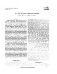
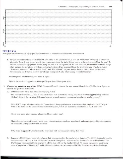
FIGURE 6.16
Blank graph for constructing the topographic profile of Problem 2. The vertical axis marks feet above sea level.
f. Being a developer of taste and refinement, you'd like to put your name in 20-foot-tall neon letters on the top of Brousseau
Mountain. But will your guests be able to see your name from the lodge dining area to be located at point X on the map? To
find out, construct a topographic profile along the line A-A' on Figure 6.15. To save time, use just the index contours except
when marking the elevations of hilltops and valley bottoms. Draw your profile on the graph provided (Fig. 6.16). Label
"Brousseau Mountain," "Great Averill Pond," and "Black Brook" on your profile. Draw a 20-foot letter on Brousseu
Mountain and see if there is a direct line of sight from point X (the future dining room) to the letter.
Will the guests be able to see your name in lights?
What is the vertical exaggeration on the profile you drew? Show your work.
3. Comparing a contour map with a DEM: Figures 6. J7 and 6.18 show the area around Mono Lake, CA. Use these figures to
answer the questions that follow.
a. Determine some basic facts about the map (Fig. 6.17):
The contour interval is 200 feet. In low-relief areas, such as in Mono Valley, they have inserted supplementary contours
(dashed). What is the elevation difference between a supplementary contour and an adjacent regular contour?
Older USGS maps often emphasize the Township and Range grid system; newer maps often emphasize the UTM grid.
What is the name for the areas outlined by the red squares, which are marked by such labels as R27E and T3 ?
About how many miles separate adjacent red lines on this map?
Maps of western states frequently show many mines (most are small and abandoned) and many springs. Draw the symbols
for mines and springs as shown on this map:
Why might mappers of western states be concerned with showing every spring they find?
b. Because I:250,000 maps cover a lot of area, their contours tend to show only larger features. The USGS sheets also tend to
be cluttered and difficult to read. In contrast, the OEM of Figure 6.18 clearly shows even subtle landscape features. The
OEM image was compiled from a series of OEMs derived from the standard USGS 7Y,-minute topographic quadrangle
maps. Comparison of Figures 6.17 and 6.18 makes obvious two advantages of OEMs: They are free of non-landscape