Topographic Maps and Digital Elevation Models
Topographic Maps and Digital Elevation Models
Topographic Maps and Digital Elevation Models

Create successful ePaper yourself
Turn your PDF publications into a flip-book with our unique Google optimized e-Paper software.
<strong>Topographic</strong> <strong>Maps</strong> <strong>and</strong> <strong>Digital</strong><br />
<strong>Elevation</strong> <strong>Models</strong><br />
Materials Needed<br />
• Pencil <strong>and</strong> eraser<br />
• Metric ruler<br />
• Calculator<br />
• <strong>Topographic</strong> quadrangle map<br />
(provided by your instructor)<br />
Introduction<br />
The topography of the Earth holds endless<br />
fascination for geologists <strong>and</strong> others who<br />
love the natural world. Topography refers<br />
to the hills, valleys, <strong>and</strong> other three-dimensional<br />
l<strong>and</strong>forms on the Earth's surface.<br />
Bathymetry refers to similar features<br />
located beneath the sea.<br />
L<strong>and</strong>scapes are interesting because<br />
they reflect the long-term action of erosional<br />
forces, such as streams, glaciers, <strong>and</strong><br />
pounding waves at the beach, <strong>and</strong> differences<br />
in how easily the underlying rocks<br />
erode. By "reading" a l<strong>and</strong>scape, geologists<br />
discover rock structures hidden beneath the<br />
soil, infer long sequences of past l<strong>and</strong>scapes,<br />
<strong>and</strong> see that the l<strong>and</strong> has uplifted or<br />
subsided. In the eyes of a geologist, a threedimensional<br />
l<strong>and</strong>scape gains the fourth<br />
dimension of time. Archaeologists familiar<br />
with natural l<strong>and</strong>forms become adept at<br />
spotting unnatural features, which helps<br />
them discover sites of ancient human<br />
activity.<br />
As you will learn in this chapter, l<strong>and</strong>scapes<br />
are conveniently visualized with<br />
the aid of maps <strong>and</strong> digital elevation models.<br />
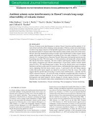
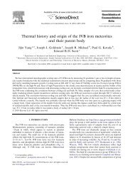
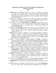
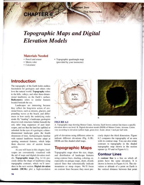
<strong>Topographic</strong> maps (Fig. 6.1A) precisely<br />
define the shape of l<strong>and</strong>forms using<br />
topographic contours, which we'll introduce<br />
in the next section. <strong>Digital</strong> elevation<br />
models (DEMs) plot a high-resolution<br />
A.<br />
FIGURE 6.1<br />
A. <strong>Topographic</strong> map showing Meteor Crater, Arizona. Each brown contour line traces a specific<br />
elevation above sea level. B. <strong>Digital</strong> elevation model (DEM) of Meteor Crater, Arizona. Colors<br />
vary according to elevation (yellow high, green low). Scale: about I inch per half mile.<br />
grid of elevations using different colors to<br />
indicate different elevations (Fig. 6.1B).<br />
DEMs are like shaded relief maps.<br />
<strong>Topographic</strong> <strong>Maps</strong><br />
<strong>Topographic</strong> maps show the size, shape,<br />
<strong>and</strong> distribution of l<strong>and</strong>scape features<br />
using contour lines, shading, coloring, or,<br />
especially on antique maps, short, closely<br />
spaced lines that schematically indicate<br />
mountains or steep slopes. We'll focus<br />
on contour lines because they most pre-<br />
B.<br />
cisely depict the third dimension. Figure<br />
6.2 compares the topography of an area<br />
with its contour map. You can also relate<br />
contours to topography in the shaded<br />
topographic map shown in the section<br />
opener (p. 93 <strong>and</strong> in Figure 6.1).<br />
Contour Lines<br />
A contour line is a line on which all<br />
points have the same elevation. It is<br />
shown in brown in Figure 6.1 A. The elevation<br />
or altitude of a point on Earth is<br />
the vertical distance between that point<br />
94
Chapter 6 <strong>Topographic</strong> <strong>Maps</strong> <strong>and</strong> <strong>Digital</strong> Elevaton <strong>Models</strong> 95<br />
Normal closed contour<br />
has same elevation as<br />
higher contour.<br />
Depression contour<br />
has same elevation<br />
as lower contour.<br />
200-foot<br />
contour<br />
Shoreline = zero-foot contour<br />
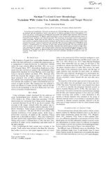
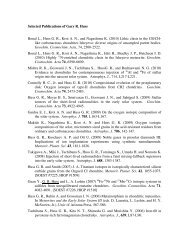
FIGURE 6.2<br />
The area sketched in the top diagram is shown as a topographic (contour) map in the bottom<br />
diagram. Contour lines (brown) on the map are drawn at intervals of 20 feet, starting with 0 at<br />
mean sea level. The fact that contours bend upstream where they cross streams allows quick<br />
recognition of hilltops. Source: U.S. Geological Survey.<br />
FIGURE 6.3<br />
A normal closed contour (above left)<br />
encircles a small hill top. If this small hill is<br />
on the side of a larger hill, the elevation of the<br />
closed contour is the same as the higher<br />
contour, as shown here.<br />
A depression contour (above right) encircles<br />
a pit or depression in the l<strong>and</strong>scape. If the<br />
depression occurs on a slope, as shown, the<br />
depression contour has the same elevation as<br />
the lower contour. With a C.I. of 10 feet, the<br />
elevation of the inner depression contour is<br />
90 feet. The bottom of the depression is less<br />
than 90 feet <strong>and</strong> more than 80 feet (because<br />
there is no 80-foot contour).<br />
<strong>and</strong> sea level, which by definition has an<br />
elevation of zero. Figure 6.2 shows an<br />
area along a sea coast, with the sea at its<br />
average elevation of zero feet. Because<br />
the edge of the shore is everywhere at an<br />
elevation of zero feet, the shoreline coincides<br />
with the zero foot contour. If sea<br />
level rose by 100 feet, the shoreline<br />
would everywhere coincide with the<br />
lOa-foot contour shown in Figure 6.2; if<br />
it rose 200 feet, it would coincide with<br />
the 200-foot contour.<br />
Contour Interval<br />
Contour lines are drawn on a map at<br />
evenly spaced intervals of elevation. The<br />
difference in elevation between two consecutive<br />
contours on the same slope is<br />
called the contour interval (C.I.). It is a<br />
constant for a given map, unless otherwise<br />
stated, <strong>and</strong> is usually given at the<br />
bottom of the map.<br />
The choice of contour interval depends<br />
on the level of detail the topographer<br />
wishes to show <strong>and</strong> the range of elevation,<br />
or relief, of the mapped area.<br />
Florida is so flat that a 5-foot contour<br />
interval often best captures the l<strong>and</strong>scape.<br />
The Rocky Mountains, on the other h<strong>and</strong>,<br />
show up best with lOa-foot contours. A<br />
5-foot interval would paint a Rockies<br />
map solid brown with over-abundant<br />
contours'<br />
Index Contours<br />
As a general rule, every fifth contour<br />
starting from sea level is an index contour.<br />
These are drawn as heavy lines <strong>and</strong><br />
labeled with their elevations (Fig. 6.2).<br />
They make it easier to read a topographic<br />
map. Contours between index contours<br />
are usually not labeled.<br />
Depression Contours<br />
Depression contours are closed contours<br />
with hachures (Sh0l1 lines perpendicular to<br />
the contour line) pointing toward the lower<br />
elevations within a depression (Fig. 6.3).<br />
They generally encircle small depressions,<br />
but can be used for large depressions (e.g.,<br />
Fig. 6.1).<br />
Contour Line<br />
Characteristics<br />
The construction <strong>and</strong> reading of contour<br />
maps are governed by the following characteristics<br />
of contour lines (most of which<br />
are illustrated in Figure 6.2):<br />
I. Every point on the same contour line<br />
has the same elevation.<br />
2. A contour line always rejoins or<br />
closes upon itself to form a loop.<br />
This may occur outside the map<br />
area. Thus, if you walked along a<br />
contour, you would eventually get<br />
back to your starting point.<br />
3. Contour lines never merge, split, or<br />
cross one another. However, if there<br />
is a steep cliff, they may appear to<br />
overlap because they are superimposed<br />
on one another.<br />
-- - -~ -~ -------=--...::~~---~~~...::==---~-- ---~-<br />
-----------
96 Part III <strong>Maps</strong> <strong>and</strong> Images<br />
4. Slopes rise or descend at right angles<br />
to any contour line.<br />
• Closely spaced contours indicate a<br />
steep slope.<br />
• Widely spaced contours indicate a<br />
gentle slope.<br />
• Evenly spaced contours indicate a<br />
uniform slope.<br />
• Unevenly spaced contours indicate<br />
a variable or irregular slope.<br />
5. Contours usually encircle a hilltop.<br />
If the hill falls within the map area,<br />
the high point will be inside the<br />
innermost contour (however, see<br />
discussion of depression contours).<br />
6. Contour lines near ridge tops or<br />
valley bottoms always occur in pairs<br />
having the same elevation on either<br />
side of the ridge or valley.<br />
7. Contours always bend upstream<br />
when they cross valleys. Because<br />
water runs downhill, this fact allows<br />
the rapid recognition of high <strong>and</strong> low<br />
areas on a contour map.<br />
8. If two adjacent contour lines have<br />
the same elevation, a change in slope<br />
occurs between them. For example,<br />
adjacent contours with the same<br />
elevation would be found on both<br />
sides of a valley bottom or ridge top.<br />
9. Depression contours have the same<br />
elevations as the normal<br />
(unhachured) contours immediately<br />
downhill (Fig. 6.3).<br />
Reading <strong>Elevation</strong>s<br />
Start with a labeled index contour. As you<br />
move uphill from this contour, keep track<br />
of the elevation by adding the value of the<br />
contour interval for every contour crossed.<br />
In Figure 6.4, moving from the 200' index<br />
contour to point X crosses two contours:<br />
200' + 20' + 20' = 240' elevation. When<br />
hiking downhill you subtract contour<br />
intervals.<br />
The elevation of a point that does not<br />
fall on a contour must be estimated. An<br />
estimate can be made by interpolation,<br />
assuming the slope between adjacent contours<br />
is uniform. For example, a point onequarter<br />
of the way between contours with<br />
elevations of 200 <strong>and</strong> 220 feet (C.l. = 20<br />
feet) would have an elevation of about<br />
205 feet. However, slopes are often not<br />
~----------200---<br />
c.\. = 20 feet<br />
FIGURE 6.4<br />
Reading elevations from a contour map with a contour interval of 20 feet. The elevation of X is<br />
240 feet, because X falls on a contour with that elevation. Point Y falls between the 240- <strong>and</strong><br />
260-foot contours, so its elevation must be between those values. Its horizontal position is about<br />
three-quarters of the way between the two, so assuming a uniform slope gives an estimated<br />
elevation of 255 feet. Point Y has a halfway elevation of 250 ± 10 feet: 250 is halfway between<br />
240 <strong>and</strong> 260, <strong>and</strong> ± 10 indicates that Y falls between 240 (250 - J0) <strong>and</strong> 260 (250 + 10). Note<br />
that the error term (± 10) is found by dividing the contour interval by two. What is the halfway<br />
elevation of Z at the top of the hill? (Answer: 310 ± 10 feet)<br />
uniform, so another approach is to give the<br />
halfway elevation between the two contours.<br />
A halfway elevation is the elevation<br />
halfway between the values of adjacent<br />
contours; thus, the elevation of a point<br />
between contours can be stated as the<br />
halfway elevation plus or minus one-half<br />
the contour interval. Figure 6.4 provides<br />
examples.<br />
Study of Figure 6.3 shows that a normal<br />
closed contour that lies between a<br />
higher <strong>and</strong> a lower contour always takes<br />
the same elevation as the higher one. A<br />
depression contour in the same situation<br />
always takes the same elevation as the<br />
lower one.<br />
<strong>Digital</strong> <strong>Elevation</strong><br />
<strong>Models</strong><br />
A digital elevation model (DEM) consists<br />
of a high-resolution grid of points<br />
assigned elevations <strong>and</strong> colored according<br />
to elevation (Fig. 6.1 B). Most DEMs<br />
are compiled from existing topographic<br />
maps. However, radar data from the<br />
Space Shuttle (SRTM), specially commissioned<br />
aircraft flights, <strong>and</strong> data from<br />
various satellites are processed to provide<br />
higher-resolution DEMs than are otherwise<br />
available from such government<br />
agencies as the U.S. Geological Survey,<br />
the Centre for <strong>Topographic</strong> Information<br />
(Natural Resources Canada), <strong>and</strong> INEGI<br />
in Mexico.<br />
DEMs make it easier to visualize<br />
l<strong>and</strong>scapes, <strong>and</strong> they often highlight subtle<br />
features that are not obvious on topographic<br />
maps. However, unless you have<br />
a computer h<strong>and</strong>y, topographic maps are<br />
more useful in the field because it is<br />
easier to read accurate elevations, spot<br />
places that are easier or more challenging<br />
to hike over, <strong>and</strong> find such hum<strong>and</strong>esigned<br />
cultural features as roads,<br />
buildings, dams, <strong>and</strong> political boundaries.<br />
If you have access to Geographic Information<br />
System (GIS) software, you can<br />
drape (superimpose) a variety of topographic<br />
map features over your DEM to<br />
get the best of both worlds.<br />
Working with <strong>Maps</strong><br />
We have to cover a few "necessary<br />
evils" before we can dive into l<strong>and</strong>scapes<br />
<strong>and</strong> topographic maps. Coordinate<br />
systems are important because they<br />
allow us to precisely locate points on<br />
the Earth's surface. We also must<br />
underst<strong>and</strong> the scale of a map so we can<br />
tell how big things are. For example, the<br />
scale of the map in Figure 6.1 A tells us<br />
that Meteor Crater is about I ~ miles<br />
across <strong>and</strong> not 50 miles across. Coordinate<br />
systems <strong>and</strong> scale are not difficult<br />
to underst<strong>and</strong> once you get used to<br />
them, but they will take some extra concentration<br />
as you read the next few sections.<br />
Underst<strong>and</strong>ing these concepts is
Chapter 6 <strong>Topographic</strong> <strong>Maps</strong> <strong>and</strong> <strong>Digital</strong> Elevaton <strong>Models</strong> 97<br />
also important if you plan on taking a<br />
GIS class in the future.<br />
Map Coordinates<br />
<strong>and</strong> L<strong>and</strong><br />
Subdivision<br />
Coordinate systems provide a permanent<br />
way of describing locations. For example,<br />
older descriptions of mineral or fossil sites<br />
commonly refer to l<strong>and</strong>marks. Unfortunately,<br />
some of these old sites are now lost<br />
because road intersections, houses, small<br />
bridges, old trees, <strong>and</strong> railway lines have<br />
since been moved or removed due to<br />
ongoing development. A coordinate system<br />
allows a state to efficiently <strong>and</strong> pennanently<br />
keep track of the locations of ab<strong>and</strong>oned<br />
oil wells, toxic waste sites, sealed<br />
mine shafts, <strong>and</strong> places hosting endangered<br />
plants or breeding pairs. It allows<br />
geologists to describe important rock<br />
localities, <strong>and</strong> it allows hikers to precisely<br />
locate trailheads, remote camp sites, <strong>and</strong><br />
other places worth remembering.<br />
Latitude-Longitude<br />
System<br />
The most well-known global coordinate<br />
system is based on east-west lines called<br />
lines of latitude <strong>and</strong> north-south lines<br />
called lines of longitude.<br />
Latitude measures distance north or<br />
south of the equator. The lines of latitude,<br />
also called parallels, form a series of parallel<br />
circles running east-west (horizontally)<br />
around the globe. The equator represents<br />
the 0° latitude line. Other parallels<br />
are set at angular intervals measured<br />
north or south of the equator, as shown in<br />
Figure 6.5A. A latitude line 40° north of<br />
the equator is termed 40° N. The geographic<br />
poles are at 90° <strong>and</strong> 90° S.<br />
Longitude measures distance east or<br />
west of the Prime Meridian. Lines of longitude,<br />
also termed meridians, form a<br />
series of circles running north-south (vertically)<br />
<strong>and</strong> intersecting at the geographic<br />
poles. The Prime Meridian is the northsouth<br />
line passing through the Royal<br />
Observatory in Greenwich, Engl<strong>and</strong>; it is<br />
defined as 0° longitude. The other meridians<br />
are set at angular intervals east or<br />
west of the Prime Meridian, as shown in<br />
A.<br />
Equator<br />
860<br />
(<br />
,J r<br />
1--' _ \<br />
J C'\ i21"...<br />
\ )/1:925 .'V \!.Y<br />
U ( r \) _ _ ~ 936<br />
B II N-r/ eRE E K<br />
/ ~ J<br />
\ I t././ -' -'<br />
T 114 N<br />
T 113 N<br />
----''----'-~<br />
~"__'___t'_----'L----'----'-L----'--'---~-JU..L-----'--LL'---'~-----''-'--L.~-=='''--~., -44°37'30"<br />
• INTERIOR-GEOLOGICAL SURVEY RESTON V1AGtN1A-1982 93037'30"<br />
'50 00om E<br />
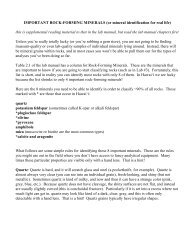
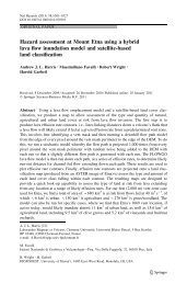
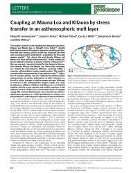
FIGURE 6.6<br />
This corner of a quadrangle map shows the latitLIde <strong>and</strong> longitude of its southern <strong>and</strong> eastern boundaries, UTM grid coordinates, <strong>and</strong> township <strong>and</strong><br />
range designations (red). The UTM grid is shown with thin black lines. Along the side, 49 45 is shorth<strong>and</strong> for 4,945,000 mN <strong>and</strong> 49 43 000 mN for<br />
4,943,000 mN. Similarly. along the bottom, 4 48 is shorth<strong>and</strong> for 448,000 mE <strong>and</strong> 4 50 000 mE for 450,000 mE. On a full-sized map, the zone number<br />
is found in the lower left corner in the fine print. This map falls within zone 15.<br />
UTM example: A given house (small black square) falls within a 1000-m square defined by grid lines 4,942,000 mN (south side), 4,943,000 mN<br />
(north), 449,000 mE (west), <strong>and</strong> 450,000 mE (east). To determine its coordinates, measure in millimeters the distance from the 4,942,000 mN line to<br />
the house <strong>and</strong> then the total distance to the 4,943,000 mN line. The house is located 39 mm out of a total 42 mm between grid lines. [n percent,<br />
39/42 = 0.93 or 93%. Since the grid distance represents 1000 m, the house is located 0.93 X 1000 = 930 m above the southern line, or at<br />
4,942,930 mN. Similarly, the house is located 20 mm/42 mm or 48% of the way east of the 449,000 mE line. This equals 449,480 mE. The location<br />
of the house, to within a 10-m square, is formally given as: 4,942.930 mN; 449,480 mE; Zone 15; northern hemisphere.<br />
98
Chapter 6 <strong>Topographic</strong> <strong>Maps</strong> <strong>and</strong> <strong>Digital</strong> Elevaton <strong>Models</strong> 99<br />
96" 95" 94" 93" 92" 91" 90" W<br />
48°N -rt-+--++--+---4+--+--t-r-~<br />
5,400,000 mN<br />
5,300,000 mN<br />
-+-+-+--+1--+--++--+-+-+ 5,200,000 mN<br />
+-+--+---++--1--++--+-+-+ 5,100,000 mN<br />
lambert Equal Area Projection<br />
A.<br />
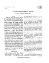
FIGURE 6.7<br />
A. UTM-grid zones in North America. Each zone is 6° of latitude wide. The<br />
zones are numbered counting west to east from the International Date Line.<br />
At the middle of each zone is the central meridian used to set up the eastwest<br />
1000-meter UTM grid lines.<br />
B. Example showing two parts of the UTM grid for zone 15 (black lines).<br />
The lines of latitude <strong>and</strong> longitude are in red. The grid system counts<br />
meters north of the equator <strong>and</strong> east or west of the central meridian, which<br />
is arbitrarily set to 500,000 meters. The lines on the two grids are parallel<br />
near the equator but not at higher latitudes because most latitude <strong>and</strong><br />
longitude lines are projected as curves, whereas UTM lines are drawn as<br />
straight lines on this projection. The point in the shaded area is located in<br />
Figure 6.6.<br />
+-+-+--I-I--+---+t----+---+--+ 5,000,000 mN<br />
44°N -~:t:t=:=+t==t:=:tt:=~:::t:4,900,000 mN<br />
! I<br />
II<br />
w E<br />
o<br />
,8<br />
I~<br />
w Eo<br />
.........~r'--, ;-,<br />
I I ' ! ,<br />
w J.J ~ 'w<br />
E E E E<br />
8 8 § g<br />
8 8 8' g\<br />
1.0 (0 I'-- co,<br />
10<br />
o<br />
/8 "<br />
+-+--++---++--+---j-+---1-+-+-+- 400,000 mN<br />
-+-+---1-j---+I---+---++--H--+--+- 300,000 mN<br />
2°N --=l:::t=ti=:tt:=::j::=~=t:t=::j:::t 200,000 mN<br />
-+-+---1-+--++---+---++--H--+--+- 100,000 mN<br />
91"<br />
90" W<br />
Because the Earth is round, even small<br />
areas (like the shaded one in Fig. 6.5B)<br />
represent curved surfaces that must be<br />
shown on flat maps. This requires a projection<br />
of the three-dimensional curved surfaces<br />
onto a two-dimensional sheet of<br />
paper. Many ways have been developed to<br />
accomplish this-names such as "Mercator<br />
projection" or "polyconic projection" may<br />
be familiar to you-but all unavoidably<br />
result in some sort of distortion <strong>and</strong> create<br />
certain difficulties.<br />
Universal Transverse<br />
Mercator (UTM)<br />
System<br />
A second widely used global coordinate<br />
grid is the UTM system. Its set-up may<br />
seem somewhat complex, but the UTM<br />
system produces a h<strong>and</strong>y grid of I-km<br />
squares on many maps. This makes it<br />
easy to determine accurate grid coordinates<br />
from paper maps <strong>and</strong> to determine<br />
distances between points. Most global<br />
positioning system (GPS) units allow you<br />
to switch between latitude-longitude <strong>and</strong><br />
UTM coordinates.<br />
The UTM system divides the 360°<br />
range of longitude into 60 north-south<br />
zones, each 6° wide. Figure 6.7A shows<br />
these zonc:s in North America. The<br />
zones are numbered from west to east,<br />
beginning at the International Date<br />
Line. The zone number is given in fine<br />
print in the lower left corner of USGS<br />
quadrangle maps. Each zone is divided<br />
into a grid with its origin at the intersection<br />
of the equator <strong>and</strong> its own<br />
central meridian, as shown for zone IS<br />
in Figure 6.7B (e.g., 93° W is the central<br />
meridian between 90° to 96°). A<br />
metric grid, with lines intersecting at<br />
right angles, is developed from this origin<br />
on a transverse-Mercator-type map<br />
projection. Lines running east-west<br />
count the number of meters from the<br />
equator. North-south lines measure the<br />
number of meters from their zone's<br />
central meridian, which is arbitrarily set<br />
to a value of 500,000 m to avoid coordinates<br />
with negative numbers (study<br />
Fig.6.7B).<br />
Features are located by their UTM<br />
coordinates. UTM coordinates are given<br />
by distinctive numbers (e.g., 49 44°00,<br />
49 45) along the margins of USGS maps<br />
(Fig. 6.6). The numbers give the distance<br />
in meters from the zone origin. In Figure<br />
6.6, for example, 49 43°00 mN describes an<br />
east-west line 4,943,000 m (4943 km)<br />
north of the equator. The east-west line<br />
I km (1000 m) to the north is 49 44°00 mN.<br />
The larger "44" makes it easier to count<br />
the I-km increments. The complete UTM<br />
coordinate is given as: north-south coordinate<br />
(northings), east-west coordinate<br />
(eastings), zone number, <strong>and</strong> hemisphere<br />
(north or south). Because some give the<br />
east-west coordinates first <strong>and</strong> the northsouth<br />
coordinates second, it is essential to<br />
label your UTM coordinate numbers with<br />
"mN" (meters north) <strong>and</strong> "mE" (meters<br />
east). Figure 6.6 gives a worked example<br />
determining UTM coordinates.
100 Part III <strong>Maps</strong> <strong>and</strong> Images<br />
A.<br />
R4E<br />
B.<br />
Correction<br />
line<br />
}Tier<br />
3S (T3S)<br />
\Correction<br />
line<br />
SE)4, NW)4, Sec. 16, T3S, R4E<br />
NW)4<br />
NW)4<br />
FIGURE 6.8<br />
U.S. Public L<strong>and</strong> Survey subdivision, illustrated by successively smaller areas. A. Example of a<br />
baseline <strong>and</strong> principal meridian in the western United States. The area to which they apply is<br />
shaded. B. From a starting point at the intersection of a principal meridian <strong>and</strong> a baseline, 6-milewide<br />
tier <strong>and</strong> range b<strong>and</strong>s subdivide l<strong>and</strong> into 36-square-mile townships. C. Townships are<br />
subdivided into 36 I-square-mile sections. D. Sections can be divided into halves, quarters,<br />
eighths, or other fractions.<br />
R5E<br />
24 T2S<br />
~ G 29<br />
31 32 33 34 35 36<br />
3 ?- /( 6 5 4 3 2 1 6 lE<br />
V 12 7 8 9 10 11 12 7<br />
,<br />
-fa 18 17 16 15 14 13 18<br />
T3S<br />
R4E<br />
~ 24 19 20 21 I~~ 24 19 A<br />
C.<br />
Wyoming<br />
R3E<br />
Base<br />
Colorado<br />
South<br />
Dakota<br />
Nebraska<br />
line<br />
Kansas<br />
T3S<br />
1""- 25 30 29 28 27 26 § ;::::-..<br />
I~ 31 32 33 34 35 36 31 tt-<br />
-?..><br />
:q 6 5 ~ 3 2 1 F<br />
--¥ H 0 T4S<br />
u.s. Public L<strong>and</strong><br />
Survey System<br />
The U.S. Public L<strong>and</strong> Survey System was<br />
designed to efficiently describe areas of<br />
l<strong>and</strong> in most states outside of the original<br />
13 colonies. This system, commonly called<br />
the Township-Range system, was started in<br />
1785, when the old Northwest Tenitory<br />
(Lake Superior region) was opened to<br />
homesteading. It has been widely used for<br />
ordinary <strong>and</strong> legal l<strong>and</strong> descriptions in the<br />
western two-thirds of the United States<br />
ever since. The method subdivides l<strong>and</strong><br />
into 6- X 6-mile squares called townships;<br />
these are further subdivided into 1- X<br />
I-mile squares called sections.<br />
D.<br />
E~<br />
The starting point for subdivision is<br />
the intersection of selected latitude <strong>and</strong><br />
longitude lines. The starting latitude is the<br />
baseline, <strong>and</strong> the starting longitude is the<br />
principal meridian. Baselines <strong>and</strong> principal<br />
meridians are established for a number<br />
of areas in the United States; an<br />
example is shown in Figure 6.8A. Lines<br />
drawn 6 miles apart <strong>and</strong> parallel to the<br />
baseline form east-west rows called tiers.<br />
North-south lines parallel to the principal<br />
meridian <strong>and</strong> 6 miles apart form northsouth<br />
columns called ranges (Fig. 6.8B).<br />
The squares formed by the intersection of<br />
tiers <strong>and</strong> ranges are called townships.<br />
Each township is approximately 6 miles<br />
square <strong>and</strong> has an area of about 36 square<br />
miles. Political townships, usually named<br />
after the largest town within the area at<br />
the time they were designated (for example,<br />
Baraboo Township, Wisconsin), may<br />
or may not coincide with Public L<strong>and</strong><br />
Survey townships.<br />
Tiers <strong>and</strong> ranges are numbered by reference<br />
to the baseline <strong>and</strong> principal meridian<br />
(Fig. 6.8B). The first tier north of the<br />
baseline is Tier 1 North (abbreviated TIN);<br />
one in the fifth tier to the north is T5N, <strong>and</strong><br />
so forth. Ranges are numbered to the east<br />
of the principal meridian (for example,<br />
R5E) <strong>and</strong> to the west (R2W). A Public<br />
L<strong>and</strong> Survey township (like the shaded one<br />
in Fig. 6.8B) is located using tier-range<br />
coordinates: T3S, R4E. NOTE: Tier is<br />
always written first, range second.<br />
Because lines of longitude (meridians)<br />
converge toward the poles, it is<br />
impossible to maintain squares that are<br />
6 miles on a side. Thus, a correction is<br />
made at every fourth tier line (labeled correction<br />
line on Fig. 6.8B), <strong>and</strong> new range<br />
lines 6 miles apart are established. The<br />
cOlTection restores townships immediately<br />
north of the line to their proper size.<br />
Each 6-mile-square township is subdivided<br />
into thirty-six, 1- X I-mile squares,<br />
called sections, which are numbered in a<br />
specific sequence (Fig. 6.8C). Each section<br />
consists of 640 acres. A section is subdivided<br />
into halves, quarters, eighths, sixteenths,<br />
<strong>and</strong> so on (Fig. 6.8D). A sixteenth<br />
of a section is 40 acres.<br />
Points are located according to the<br />
smallest subdivision required. In Figure<br />
6.8D, the star is located, to the nearest<br />
40 acres, in the SE )4, NW )4, Sec. 16,<br />
T3S, R4E. Locations are always written<br />
from the smallest unit to the largest, <strong>and</strong><br />
tier is written before range.<br />
Section numbers <strong>and</strong> tier <strong>and</strong> range<br />
values are written in red on USGS topographic<br />
maps (see Fig. 6.6).<br />
Map Scale<br />
The scale of a map is essential because it<br />
tells the user the size of the area represented<br />
<strong>and</strong> the distance between various<br />
points. Three types of scales are in common<br />
use: ratio, graphic, <strong>and</strong> verbal scales.<br />
A ratio or fractional scale, shown at<br />
the bottom of Figure 6.9, is the ratio<br />
between a distance on a map <strong>and</strong> the<br />
actual distance on the ground. The ratio
U.S. Public L<strong>and</strong> Survey<br />
Range coordinate<br />
r<br />
Intermediate<br />
longitude<br />
(in minutes <strong>and</strong> seconds)<br />
rUTM coordinate<br />
(without zeros;<br />
kilometers east)<br />
MT. SHASTA QUADRANGLE<br />
CAUFORNIA -- SISKIYOU CO.<br />
7.5 MINUTE SERIES (TOPOGRAPHIC)<br />
U.S. Public<br />
L<strong>and</strong> Survey<br />
tiercoo~<br />
U.S. Public<br />
L<strong>and</strong> Survey ~<br />
section number/' -<br />
StatePla~<br />
coordin~t~" ~<br />
number (not<br />
discussed)<br />
Map data,<br />
including UTM<br />
......-.s-"""'-......'_<br />
zone <strong>and</strong> the '=.~~~":.__ _ \V _<br />
North :2-=::?:::'-:7-_ 1~ 11.5._. 8 =~----<br />
American _....:::-~.::.:.:=..-=.-_"';';' 13 -----<br />
Datum to use ~::.:::=E:.:::r=:-: ...L~~==:::;;:-""""t__;::=:;::'~=~~::::':'::~~=-_;:::±:;:=7"""rrl"'T'J"T'J:~~ .__ 0 ::;"---- ---<br />
in your GPS _=~:'::J::.:""':__~. Contour • :::::..-- :::-'::~:-""a ~ ==-<br />
FIGUR~e:~;er.\. ~...:=;:...-::.::..-:.:==;=.- ,',:-. ";'':: ~ interval • !~~~-::=C MT. S~A, CA )<br />
"'--J Magnetic declination Names of ,--..- t<br />
Reduced copy of the Mt. Shasta, California, 7'/,- (MN) adjoining---... '-----t--+---I~=--<br />
d I r- 6CllyofMt.Sh-.<br />
minute quadrangle, with principal map features qua rang es ~~ Name of quadrangle<br />
highlighted <strong>and</strong> magnified. """'""""". <strong>and</strong> year of publication<br />
101Xll
102 Part III <strong>Maps</strong> <strong>and</strong> Images<br />
scale on Figure 6.9 is I:24,000 (or<br />
1124,000), which means that one unit (for<br />
example, an inch) on the map equals<br />
24,000 of the same units on the ground.<br />
A graphic scale usually consists of a<br />
scale bar subdivided into divisions corresponding<br />
to a mile or kilometer (see Fig.<br />
6.9). One mile or kilometer segment on<br />
the scale bar is commonly subdivided to<br />
allow more precise measurements of distance.<br />
The subdivided units are commonly<br />
placed to the left of zero on a scale bar, as<br />
in Figure 6.9. A graphic scale is helpful<br />
because it is readily visualized <strong>and</strong> stays<br />
in true proportion if the map is enlarged or<br />
reduced. It also provides a convenient way<br />
of measuring distances between points on<br />
a map: lay a strip of paper between the<br />
points <strong>and</strong> make pencil marks next to<br />
each point. Then lay the paper along the<br />
graphic scale at the bottom of the map <strong>and</strong><br />
determine the distance.<br />
A verbal scale is commonly used to<br />
discuss maps but is rarely written on<br />
them. People usually say, "I inch equals<br />
I mile," which means, "I inch on the map<br />
represents, or is proportional to, 1 mile<br />
on the ground." Because I mile equals<br />
63,360 inches, a common fractional scale<br />
of 1:62,500 on older maps corresponds<br />
closely to the verbal scale "I inch to<br />
I mile." Many U.S. maps, <strong>and</strong> essentially<br />
all foreign maps, use metric scales, making<br />
common fractional scales easily convertible<br />
to verbal scales: scales of<br />
I:50,000, I: 100000, <strong>and</strong> I:250,000 correspond<br />
to I centimeter equaling 0.5, 1.0,<br />
<strong>and</strong> 2.5 kilometers, respectively.<br />
4° quadrangle maps are drawn at a<br />
fractional scale of I: I,000,000; 2° quadrangles<br />
at I:500,000; I° at I:250,000; 15' at<br />
I:62,500 or I:50,000; <strong>and</strong> 7'.1.' at 1:24,000<br />
or 1:25,000. Both graphic <strong>and</strong> fractional<br />
scales are shown at the bottom center of the<br />
map (see Fig. 6.9).<br />
These different scales are used to<br />
show larger or smaller areas of the Earth's<br />
surface on conveniently sized maps. For<br />
example, it may be possible to show a<br />
small city on a map where I inch on the<br />
map represents 12,000 inches (1000 ft) on<br />
the ground. This map would have a scale<br />
of I: 12,000. However, to show a midsized<br />
state, such as Indiana, on a map of<br />
similar size, the scale would have to be<br />
much smaller, say I inch on the map to<br />
500,000 inches (approximately 8 miles) on<br />
the ground. In general, the larger the area<br />
shown, the smaller the scale of the map<br />
(smaller because the fraction 1!500,000 is<br />
a smaller number than 1/12,000).<br />
Converting Among<br />
Scales<br />
Verbal to fractional scale<br />
conversion:<br />
I. Convert map <strong>and</strong> ground distances<br />
to the same units.<br />
2. Write the verbal scale as the fraction:<br />
I. Convert both map <strong>and</strong> ground distances<br />
to the same units, inches:<br />
5000 X 12" = 60,000". The verbal<br />
scale is now 2.5 inches on the map<br />
represents 60,000 inches on the<br />
ground.<br />
2. Write the verbal scale as the fraction:<br />
2.5" (distance on map)<br />
60,000" (distance on ground)<br />
3. Divide the numerator <strong>and</strong> denominator<br />
by the value of the numerator:<br />
2.5"/2.5"<br />
60,000"/2.5"<br />
Distance on map<br />
Distance on ground<br />
3. Divide both numerator <strong>and</strong> denominator<br />
by the value of the numerator:<br />
Distance 0/1 map/distance on map<br />
Distance on ground/distance on map<br />
Example: Convert the following verbal<br />
scale to a fractional scale: 2.5 inches on<br />
the map represents 5000 feet on the<br />
ground.<br />
I<br />
24,000 or 1:24,000<br />
Fractional to verbal scale<br />
conversion:<br />
I. Select convenient map <strong>and</strong> ground<br />
units to relate to each other (for<br />
example, inches <strong>and</strong> miles or centimeters<br />
<strong>and</strong> kilometers).<br />
2. Express fractional scale using the<br />
map units (inches or centimeters).<br />
3. Convert the denominator to the<br />
ground units (miles or kilometers).<br />
4. Express verbally as "I inch [or<br />
I centimeter] equals X miles [or<br />
kilometers]."<br />
Example: Convert a fractional scale of<br />
I:62,500 to a verbal scale of I map inch<br />
equals X miles on the ground.<br />
I. Units to be related are inches <strong>and</strong><br />
miles.<br />
2. 1:62,500 = 1"/62,500"<br />
3. Convert 62,500" into miles by dividing<br />
by the number of inches in<br />
I mile. One mile = 5280 feet <strong>and</strong><br />
1 foot = 12 inches. So, 1 mi =<br />
5280' X 12" = 63,360". Working<br />
out the division:<br />
62,500 inches .<br />
63 360 ' I . = 0.986111/<br />
, mc 1es per 1111<br />
4. Expressed verbally, I inch on the<br />
map equals 0.986 mile on the<br />
ground.<br />
Magnetic<br />
Declination<br />
<strong>Maps</strong> are usually drawn with north at<br />
the top. North on a map refers to true<br />
geographic north. At most places on<br />
Earth, however, a compass needle does<br />
not point toward the geographic north<br />
pole but toward the magnetic north pole.<br />
The magnetic north pole is in the<br />
Canadian Arctic, but its exact position<br />
changes. For example, in 1955, it was<br />
located north of Prince of Wales Isl<strong>and</strong><br />
near latitude 74° N, longitude 100° W;<br />
its last measured location in 200 I put it<br />
in the Canadian Arctic Ocean (81.3° N,<br />
110.3° W) headed northwest toward<br />
Siberia at 40 km/year.<br />
The angular distance between true<br />
north <strong>and</strong> magnetic north is the magnetic<br />
declination. Because the location<br />
of the magnetic pole changes, the magnetic<br />
declination generally varies with<br />
time. If you are navigating or doing geologic<br />
research using a compass, you<br />
must adjust the declination of the compass<br />
for local conditions. Without<br />
adjustment, compass errors in excess of<br />
10° to 20° are possible along the west<br />
<strong>and</strong> east coasts of North America! The<br />
magnetic declination is shown at the<br />
bottom of most USGS maps by two<br />
arrows (see Fig. 6.9). One points to true<br />
north (commonly marked with a star, or<br />
T.N.) <strong>and</strong> one points toward magnetic<br />
north (commonly marked M.N.). The
Chapter 6 <strong>Topographic</strong> <strong>Maps</strong> <strong>and</strong> <strong>Digital</strong> Elevaton <strong>Models</strong> 103<br />
angular separation between them (the<br />
magnetic declination) also is given.<br />
When stating the magnetic declination<br />
of a map, it is always necessary to indicate<br />
whether the arrow pointing to the<br />
magnetic pole is east or west of the geographic<br />
pole. If it is east, the declination<br />
is stated as so many degrees east, for<br />
example, 212° E. Most maps also have<br />
an arrow pointing toward G.N., the<br />
location of the grid north direction for<br />
the Universal Transverse Mercator<br />
(UTM) grid system (see Fig. 6.9).<br />
Symbols<br />
St<strong>and</strong>ardized symbols <strong>and</strong> colors are used<br />
on government maps to designate various<br />
features. On USGS maps, cultural features<br />
(those made by people) are generally<br />
drawn in black; forests or woods are<br />
shown in green (they are not always represented);<br />
blue is used for bodies of<br />
water; brown shows elevation (contours),<br />
some mining operations, <strong>and</strong> beaches or<br />
s<strong>and</strong> areas; <strong>and</strong> red is used for the better<br />
roads <strong>and</strong> some l<strong>and</strong> subdivision lines.<br />
See Figure 6.10 for symbols <strong>and</strong> Figure<br />
6.9 for some examples. Note that when<br />
USGS topographic maps are revised, any<br />
new features (e.g., roads, suburbs, strip<br />
mines) that appear in an area are colored<br />
purple. Symbols for Canadian government<br />
maps are shown on the backs of the<br />
maps. Mexican map symbols are generally<br />
on the front.<br />
Working with<br />
<strong>Topographic</strong> <strong>Maps</strong><br />
Now that you underst<strong>and</strong> contours, coordinate<br />
systems, <strong>and</strong> scale, we are ready to<br />
cover some ways of working with topographic<br />
maps. We'll start with the basics<br />
of how topographic maps are produced.<br />
Making <strong>Topographic</strong><br />
<strong>Maps</strong><br />
Making a topographic map requires accurate<br />
points of elevation in the map<br />
area. A bench mark is a point whose<br />
elevation <strong>and</strong> location have been precisely<br />
determined by government surveyors;<br />
its location is marked by a small<br />
brass plate. Bench marks are designated<br />
on maps by the symbol B.M. (Fig. 6.9).<br />
Spot elevations are somewhat lessprecisely<br />
determined elevations used in<br />
the construction of topographic maps.<br />
They are shown at many section corners,<br />
bridges, road intersections, hilltops,<br />
<strong>and</strong> the like <strong>and</strong> may be marked<br />
with an "x" (examine Fig. 6.9). Bench<br />
marks <strong>and</strong> spot elevations are used in<br />
conjunction with aerial photographs to<br />
construct topographic maps. Two aerial<br />
photos, taken from different points but<br />
overlapping the same area, provide a<br />
three-dimensional view of the l<strong>and</strong> surface<br />
when viewed through a stereoscopic<br />
viewer. By orienting the photos properly,<br />
two beams of light from different<br />
sources can be focused at any elevation.<br />
If the superimposed beams are moved<br />
around a hill, for example, they will<br />
trace a line at a precise elevation. The<br />
numerical value of this elevation can<br />
be determined from known elevations<br />
within the area (e.g., bench marks). Aerial<br />
photographs are discussed further in<br />
Chapter 7.<br />
If you are a l<strong>and</strong>scaper or an architect,<br />
for example, you may want to make<br />
your own detailed topographic map of an<br />
area. You can start by tracing any important<br />
features (drainages, coastlines,<br />
buildings, etc.) from an air photo<br />
obtained from the USGS or from your<br />
state. Then, starting from the lowest spot<br />
on the property, take a series of hikes<br />
uphill with a 5-foot staff <strong>and</strong> a spirit<br />
(bubble) level that allows you to site<br />
horizontal lines from the top of your<br />
staff. These allow you to plot successive<br />
elevation increments of 5' on your map<br />
(Fig. 6.l1A). Now add the contours to<br />
reflect the l<strong>and</strong>scape by following these<br />
steps:<br />
I. Select a contour interval that will<br />
show the level of detail you need.<br />
Too many contours can be confusing.<br />
2. If your staff was a convenient length<br />
(e.g., 5 feet), simply connect those<br />
points that correspond to multiples<br />
of the contour interval. If the c.I. is<br />
20 feet, you would connect dots<br />
marking 20, 40, 60, etc., feet.<br />
3. Draw fairly smooth, fairly parallel<br />
contours, but be sure to bend them<br />
upstream when crossing drainages<br />
<strong>and</strong> gullies (Fig. 6.l1B). Adding<br />
extra wiggles implies you know<br />
more than you do. Draw the lines to<br />
the edge of the map. Label each<br />
contour or index contour with its<br />
elevation.<br />
<strong>Topographic</strong> Profiles<br />
A topographic profile shows the shape<br />
of the l<strong>and</strong> surface as it would appear in a<br />
cross section; it is like a side view. <strong>Topographic</strong><br />
profiles portray the shape of the<br />
l<strong>and</strong> surface along a particular line of profile.<br />
They are useful for many practical<br />
purposes, such as planning roads, railroads,<br />
pipelines, hiking trails, <strong>and</strong> the<br />
like, or for estimating the volume of<br />
material that will need to be excavated or<br />
filled during road construction. Profiles<br />
are most easily made along straight lines,<br />
but they can also follow curved paths,<br />
such as a road or a stream.<br />
A topographic profile is made from a<br />
contour map using the following procedure<br />
(Fig. 6.12):<br />
l. Select the line or path along which<br />
the profile is to be made, such as line<br />
X-Y in Figure 6.l2A.<br />
2. Record the elevations along the line<br />
as shown in Figure 6.12B. To do this,<br />
lay the straight edge of some scratch<br />
paper along the line of profile. Mark<br />
on the paper the ends of the profile<br />
line <strong>and</strong> the exact place where each<br />
contour line meets the edge of the<br />
paper. Label each mark on the paper<br />
with the elevation of the corresponding<br />
contour. Also mark the positions<br />
of any streams that cross the line of<br />
profile, because they will be low<br />
points on the profile.<br />
3. Set up the graph on which the profile<br />
will be drawn (Fig. 6.l2C). First note<br />
the differences in elevation between<br />
the highest <strong>and</strong> lowest points along the<br />
line of profile; this will determine the<br />
range of elevations on your profile.<br />
Label the vertical axis with a range of<br />
elevations that extends beyond the<br />
profiJe elevations <strong>and</strong> conveniently<br />
allows each contour to be graphed. In<br />
Figure 6.l2C, the profile elevations<br />
range between 820 <strong>and</strong> 940 feet <strong>and</strong><br />
are spanned by a vertical axis of 700<br />
to 1000 feet. Horizontal lines on the<br />
vel1ical axis are 20 feet apart, which<br />
matches the contour intervaJ <strong>and</strong><br />
makes graphing simple. CommonJy,
<strong>Topographic</strong> Map Symbols<br />
BOUNDARIES<br />
RAILROADS AND RELATED FEATURES<br />
COASTAL FEATURES<br />
National. .<br />
......_-- St<strong>and</strong>ard gauge single track; station..<br />
Foreshore flat (shallow sediment).<br />
State or territorial<br />
_ St<strong>and</strong>ard gauge multiple track .<br />
Rock or coral reef .<br />
County or equivalent. --- Ab<strong>and</strong>oned .<br />
Rock bare or awash ..<br />
Civil township or equivalent.<br />
Incorporated-eity or equivalent. .<br />
.... . 1-_, _<br />
. .r- - - - -<br />
Under construction<br />
Narrow gauge single track .<br />
.<br />
Group of rocks bare or awash.<br />
Exposed wreck......................•..<br />
Park, reservation, or monument. ..<br />
.I-- . _ Narrow gauge multiple track .<br />
Depth curve; sounding .<br />
Small park .<br />
Railroad in street. .<br />
Breakwater, pier, jetty, or wharf.<br />
Juxtaposition........................•.<br />
Seawall ..<br />
LAND SURVEY SYSTEMS<br />
Roundhouse <strong>and</strong> turntable .<br />
U.S. Public L<strong>and</strong> Survey System:<br />
Township or range line.<br />
TRANSMISSION LINES AND PIPELINES<br />
BATHYMETRIC FEATURES<br />
Area exposed at mean low tide; sounding datum ._...../.<br />
Location doubtful. ... f- _ _ _ Power transmission line: pole; tower..<br />
Channel .<br />
Section line<br />
f-----j Telephone or telegraph line.<br />
Offshore oil or gas: well; platform . o •<br />
Location doubtful. --- Above-ground oil or gas pipeline.<br />
.~__~ Sunken rock.<br />
Found section corner; found closing corner I- ~ ~_ Underground oil or gas pipeline .<br />
Witness corner; me<strong>and</strong>er corner ~c1+ _ ~<br />
RIVERS, LAKES, AND CANALS<br />
I MC,<br />
CONTOURS<br />
Intermittent stream . . ....---. .<br />
Other l<strong>and</strong> surveys:<br />
<strong>Topographic</strong>:<br />
Intermittent river .<br />
..... - ..::::::<br />
Township or range line.<br />
Section line.<br />
Intermediate .<br />
Disappearing stream.<br />
.. .. ---<<br />
L<strong>and</strong> grant or mining claim; monument.. ..... +_ _ to<br />
Index .<br />
Perennial stream.<br />
Fence line ..<br />
Supplementary .<br />
Perennial river .<br />
Depression ..<br />
Small falls; small rapids .<br />
ROADS AND RELATED FEATURES<br />
Cut; fill ..<br />
I-."~"";,.j Large falls; large rapids .<br />
Primary highway..<br />
f---~ Bathymetric:<br />
Secondary highway..<br />
Intermediate.<br />
Masonry dam .<br />
Light duty road.<br />
Index.<br />
Unimproved road.<br />
Primary..<br />
Dam with lock.<br />
Trail. .<br />
Index Primary .<br />
Dual highway.<br />
Supplementary.<br />
Dual highway with median strip .<br />
Dam carrying road.<br />
Road under construction . ~_~ MINES AND CAVES<br />
Underpass; overpass.. .~ Quarry or open pit mine .<br />
Intermittent lake or pond , .<br />
Bridge . I-__~ Gravel, s<strong>and</strong>.. clay, or borrow pit. .<br />
Dry lake ..<br />
Drawbridge.<br />
I-__~ Mine tunnel or cave entrance.<br />
Narrow wash.<br />
Tunnel.<br />
. 1-0"""'- Prospect; mine shaft. .<br />
Wide wash .<br />
','<br />
Mine dump ..<br />
Canal, flume, or aqueduct with lock .<br />
BUILDINGS AND RELATED FEATURES<br />
Dwelling or place of employment: small; large.. • _<br />
Tailings .<br />
Elevated aqueduct, flume, or conduit.<br />
Aqueduct tunnel.<br />
School; church. •• SURFACE FEATURES<br />
Barn, warehouse, etc.: small; large. 0 ~ Levee<br />
Water well; spring or seep .<br />
House omission tint.<br />
S<strong>and</strong> or mud area, dunes, or shifting s<strong>and</strong>.<br />
GLACIERS AND PERMANENT SNOWFIELDS<br />
Racetrack .<br />
Intricate surface area.<br />
. >'-
Chapter 6 <strong>Topographic</strong> <strong>Maps</strong> <strong>and</strong> <strong>Digital</strong> Elevaton <strong>Models</strong> 105<br />
x<br />
15<br />
A.<br />
x<br />
x15 25<br />
x26<br />
x20 2~<br />
/<br />
23 x<br />
x 20<br />
x 15 x<br />
15 x / 20<br />
x x 10 x<br />
15 10 x<br />
/ 15<br />
x x 5 x<br />
10 5 10<br />
x<br />
x 5<br />
5<br />
A. B.<br />
FIGURE 6.11<br />
How to make a contour map: A. <strong>Elevation</strong>s from numerous transects across the area are added to<br />
a sketch map. B. Smooth contour lines connect the dots at the elevations corresponding to the<br />
contour interval. Lines are smooth except where they cross drainages.<br />
I i I i I I I I I<br />
I<br />
i i I i i i I<br />
X~ 0 0 0 0 0 0 0 0 0 0 00<br />
c;o co 0 0 co c;o<br />
E 't c;o co 0C\j<br />
co co co ~<br />
~Y<br />
0) 0) co co Cll co co co 0)0)<br />
~<br />
1000 ,---;.--+--+-+--+---;----;-----+---">--+-;--+---;..->--.---+,-----------,1000<br />
--<br />
900 1--+-+---+:-./---="'="-:::__ :---+------'f------t----...;--+--7:/---,1:"--/---+----1900<br />
:./ :/<br />
:/ --:/<br />
c.<br />
800f--------------------------jf---I800<br />
x<br />
y<br />
y<br />
4.<br />
as here, the vertical <strong>and</strong> horizontal<br />
scales are different. In Figure 6.l2C,<br />
the horizontal scale is about I" equals<br />
800' (1:9600) whereas the vertical<br />
scale is 1" equals 160' (1:1920). If the<br />
scales were the same, the profile<br />
would look flat. Use of an exp<strong>and</strong>ed<br />
vertical scale highlights (exaggerates)<br />
topographic variations.<br />
Transfer each mark made along the<br />
profile to the appropriate place on<br />
the graph paper by aligning the<br />
paper with your graph (Fig. 6.12C).<br />
Mark the ends of the profile on the<br />
graph paper. Mark the contour <strong>and</strong><br />
stream points on the graph at their<br />
appropriate elevations. This is done<br />
by going straight up from the mark<br />
on the paper (or, as illustrated here,<br />
down from the top of the graph<br />
paper with the marks made directly<br />
on it) to the horizontal line representing<br />
the same elevation; make a<br />
small dot on the paper at this point.<br />
5. Connect the points on the graph<br />
paper with a smooth line representing<br />
the topography (Fig. 6.12C).<br />
When crossing a valley or a hilltop,<br />
there will be adjacent marks with the<br />
same elevation. Instead of connecting<br />
them with a straight line, draw<br />
your profile line so it goes up over a<br />
hilltop or down into a valley. In the<br />
case of a stream valley, the low point<br />
in the valley will be where the<br />
stream crosses the line of profile.<br />
Vertical Exaggeration<br />
of <strong>Topographic</strong> Profiles<br />
Profiles are commonly drawn with a vertical<br />
scale that is larger than the horizontal<br />
scale. This vertical exaggeration reveals<br />
topographic features that otherwise might<br />
not show up on the profile. The amount of<br />
vertical exaggeration is determined by the<br />
ratio of the horizontal map scale (for<br />
FIGURE 6.12<br />
Construction of a topographic profile.<br />
A. Choose a line of profile (X-Y). B. Mark<br />
intersections of contours <strong>and</strong> the stream, <strong>and</strong><br />
note elevations on paper laid along the profile<br />
line. C. Choose a vertical scale, <strong>and</strong> transfer<br />
the points from the previous step to the<br />
appropriate elevations. Connect the points<br />
with a smooth line to complete the profile.<br />
--~----- - - ---- . ----------
106 Part III <strong>Maps</strong> <strong>and</strong> Images<br />
I H<strong>and</strong>s-On<br />
Applications<br />
You are probably already familiar with maps used to display roads <strong>and</strong> political boundaries. The h<strong>and</strong>son<br />
exercises that follow develop the basic skills needed to use <strong>and</strong> interpret the information-rich topographic<br />
maps. As you will see throughout this lab manual, such maps are essential for recognizing <strong>and</strong><br />
underst<strong>and</strong>ing the character, origin, <strong>and</strong> even future of many l<strong>and</strong>scapes. You will also see how geological<br />
data, when plotted on maps, can clearly present a picture that is difficult to see without a great<br />
deal of field work. Learn well the skills in this chapter, for they will serve you over <strong>and</strong> over again<br />
throughout this class. You will also draw upon these skills if you choose a career dealing with any<br />
aspect of the Earth's surface (e.g., in geology, environmental remediation <strong>and</strong> planning, l<strong>and</strong> use planning,<br />
archaeology, biodiversity <strong>and</strong> ecologic assessment, resources management, parks <strong>and</strong> recreation,<br />
civil engineering, etc.).<br />
Objectives<br />
If you are assigned all the prob- 6. Number the sections of a direction of stream flow, <strong>and</strong><br />
lems, you should be able to: township if they are not already locations of hills <strong>and</strong> valleys.<br />
numbered on the map.<br />
1. Define latitude <strong>and</strong><br />
13. Determine the contour interval<br />
longitude. 7. Determine the scale of a map <strong>and</strong> of a map.<br />
use it to measure distances.<br />
2. Describe the boundaries of a<br />
14. Make a topographic map using<br />
quadrangle map in terms of 8. Convert among verbal, fractional, points of elevation to draw<br />
latitude <strong>and</strong> longitude, <strong>and</strong> <strong>and</strong> graphic scales. contour lines.<br />
locate a point on a map using 9. Give the magnetic declination of IS. Construct a topographic profile<br />
these coordinates. a map (assuming it is printed on <strong>and</strong> determine its vertical<br />
3. Locate a point using the the map) <strong>and</strong> explain what it exaggeration.<br />
Universal Transverse means. 16. Detennine the gradient of a<br />
Mercator (UTM) system. 10. Determine what the various stream using a topographic map.<br />
4. Locate or describe a parcel of symbols used on a map mean<br />
l<strong>and</strong> using the U.S. Public<br />
(symbols for streams, roads,<br />
L<strong>and</strong> Survey System, <strong>and</strong><br />
houses, etc.).<br />
give its area in acres.<br />
11. Use a contour map to determine<br />
S. Give the dimensions <strong>and</strong> area elevation, height, <strong>and</strong> relief.<br />
of a section <strong>and</strong> township (in 12. Use the characteristics of contours<br />
miles <strong>and</strong> square miles).<br />
to determine steepness of slope,<br />
Problems<br />
1. The basics of USGS topographic maps: Examine the map provided by your instructor to answer the following questions. Tables<br />
to convert between different units are found inside the back cover. Show any calculations you make.<br />
a. What is the name of the quadrangle <strong>and</strong> in what year was it last published or revised?<br />
b. As frequently happens, you become interested in a feature that goes off the map. What are the names of the quadrangles to<br />
the east <strong>and</strong> southeast?<br />
107<br />
- - ----~--------- ~-
108 Part III <strong>Maps</strong> <strong>and</strong> Images<br />
c. What is the northern boundary latitude?<br />
Southern boundary latitude?<br />
Western boundary longitude?<br />
Eastern boundary longitude?<br />
Subtract these latitude <strong>and</strong> longitude numbers to get the size of the quadrangle in units of degrees, minutes, <strong>and</strong> seconds.<br />
d. What is the fractional scale of the map?<br />
Determine the approximate verbal scale: I inch =<br />
miles. As always, show your calculations.<br />
An environmental restoration project requires that you enlarge part of the map to a scale of 1 inch to 1000 feet. Calculate<br />
the factor by which it needs to be enlarged.<br />
What would the enlargement factor be if you needed a scale of 1 em to 100 m? Hint: Start with the fractional scale.<br />
e. What is the contour interval?<br />
f. What is the highest elevation within the area designated by your instructor?<br />
What is the lowest elevation in that area?<br />
What is the relief of the designated area?<br />
g. What is the height (not the elevation) of the location designated by your instructor?<br />
h. Give the elevation of the location designated by your instructor.<br />
I. Determine to the nearest minute the approximate latitude <strong>and</strong> longitude of the designated feature.<br />
j. Determine to the nearest 100 m the full UTM coordinates of the designated feature.<br />
k. If the map is subdivided by the Township-Range method, locate the feature designated by your instructor to the nearest Y,6th<br />
of a section.<br />
I. What is the approximate size of the area designated by your instructor (in acres, if subdivided by the Township-Range<br />
method, in square meters if the UTM method is preferred)?<br />
m. Use the graphic scale to determine the distance in miles <strong>and</strong> kilometers between the features designated by your instructor.<br />
n. In what direction does the water flow in the stream designated by your instructor?<br />
o. What is the magnetic declination (in degrees) indicated on the map? In which year was this value measured?
Chapter 6 <strong>Topographic</strong> <strong>Maps</strong> <strong>and</strong> <strong>Digital</strong> Elevaton <strong>Models</strong> 109<br />
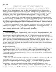
2. Analyze a l<strong>and</strong>scape: Let's say that you're a developer with a big project in mind for an area near Averill, Vermont<br />
(Fig. 6.15). You first need to study a topographic map to underst<strong>and</strong> the l<strong>and</strong>scape. Show any calculations you make for the<br />
following questions. Conversion factors are listed inside the back cover.<br />
a. Determine the following basic facts about the map:<br />
Interval between index contours:<br />
Contour interval (units in feet):<br />
Fractional scale (Hint: Use the UTM grid <strong>and</strong> metric units.):<br />
Verbal scale (I inch =<br />
miles):<br />
Approximate height <strong>and</strong> width of the map. (Hint: Use the UTM grid as a bar scale.)<br />
Approximate height <strong>and</strong> width of the map in miles (Hint: Use the verbal scale <strong>and</strong> a ruler.):<br />
By what factor was this map enlarged or reduced from its original 1:24,000 scale?<br />
b. To get a feel for the l<strong>and</strong>scape, find the three most prominent mountains rising above 2200 feet. List their elevations starting<br />
with the mountain near the top of the map <strong>and</strong> going clockwise. The "T" following the bench mark elevations means they<br />
were determined from air photo measurements, which have errors of a few feet relative to the more accurate method of<br />
surveying.<br />
c. Determine which way the streams flow by looking at how the contours are deflected as they cross them. Draw arrows<br />
showing the flow directions of the streams flowing into or out of the ponds <strong>and</strong> lake.<br />
Which ponds or lakes flow into each other? (You can double-check your inferences by noting water level [WL] elevations.)<br />
Use the stream drainages to help you find the lowest elevation on the map. What is this elevation?<br />
What is the total relief of the map area?<br />
Let's say that you plan to hike up Brousseau Mountain from a canoe beached on Little Averill Pond. What is the height of<br />
Brousseau Mountain relative to this starting point?<br />
d. At the top of Brousseau Mountain you plan on checking your h<strong>and</strong>-held Global Positioning System (GPS) unit to be sure it<br />
works. Note that UGSG maps show latitude <strong>and</strong> longitude divisions no finer than 2' 30" (see left map margin), so you have<br />
to switch your GPS unit to UTM coordinates. Use the map to determine the UTM grid coordinates you expect to see when<br />
you reach the peak of the mountain (marked with an elevation on the map).<br />
e. Because your development plans include golf courses, a water park, factory outlet shopping, <strong>and</strong> extreme paintball, you need<br />
quite a bit of l<strong>and</strong> around the Averill ponds. Do the little black dots on the map represent anything relevant to your<br />
development plans? Explain.
(<br />
FIGURE 6.15<br />
Portion of the Averill, Vermont, 7 ~-minute quadrangle<br />
map for use in Problem 2. Canada is just a few kIn north<br />
of the map area. Scale <strong>and</strong> contour interval are determined<br />
as part of Problem 2.<br />
110
Chapter 6 <strong>Topographic</strong> <strong>Maps</strong> <strong>and</strong> <strong>Digital</strong> Elevaton <strong>Models</strong> III<br />
o -------------.-----------------------------..------- .. --------..--------.---------------------------.----------------------------.-----------------.------------------------------------.--------------------------.----------------.-------------------------<br />
55-----------------------------------------------------.-.--...---- ..-.....----- ..--- ....-------------------------------------------<br />
C\J -------------.--••••••••-•• -••• -.-.-.---------.-------••• --------.-------•• -------- •• -------•• -------- •• --------.-------- •• --------.-------- •• ------ •• ------- •• --------.-- ----- •• --------.-------•• --------.--------.--------.-------•••• -------.-------<br />
o ---- --- ------.--------.-.-- - --.--.- -.---- - ----- -..---........... ----.- - -------.--- - ---- .<br />
8- ---.-------------..--.------ -..------------------------------------------------------------------------------------------------<br />
C\J ••••••••••••••••••-•••••••••••••••••••••••••••••••••••••••••••••••••••••••-.---.---.--••••••••-•• -••• ----------------.--•• ----. --------.--------.-.------.-------- •• ------- •• --- •• -••• --------. --------•• -- •••••••• -•••••• ----------------••••••••-.-••• --<br />
o<br />
55 .......---------------------------------------------------'<br />
~A<br />
A'<br />
FIGURE 6.16<br />
Blank graph for constructing the topographic profile of Problem 2. The vertical axis marks feet above sea level.<br />
f. Being a developer of taste <strong>and</strong> refinement, you'd like to put your name in 20-foot-tall neon letters on the top of Brousseau<br />
Mountain. But will your guests be able to see your name from the lodge dining area to be located at point X on the map? To<br />
find out, construct a topographic profile along the line A-A' on Figure 6.15. To save time, use just the index contours except<br />
when marking the elevations of hilltops <strong>and</strong> valley bottoms. Draw your profile on the graph provided (Fig. 6.16). Label<br />
"Brousseau Mountain," "Great Averill Pond," <strong>and</strong> "Black Brook" on your profile. Draw a 20-foot letter on Brousseu<br />
Mountain <strong>and</strong> see if there is a direct line of sight from point X (the future dining room) to the letter.<br />
Will the guests be able to see your name in lights?<br />
What is the vertical exaggeration on the profile you drew? Show your work.<br />
3. Comparing a contour map with a DEM: Figures 6. J7 <strong>and</strong> 6.18 show the area around Mono Lake, CA. Use these figures to<br />
answer the questions that follow.<br />
a. Determine some basic facts about the map (Fig. 6.17):<br />
The contour interval is 200 feet. In low-relief areas, such as in Mono Valley, they have inserted supplementary contours<br />
(dashed). What is the elevation difference between a supplementary contour <strong>and</strong> an adjacent regular contour?<br />
Older USGS maps often emphasize the Township <strong>and</strong> Range grid system; newer maps often emphasize the UTM grid.<br />
What is the name for the areas outlined by the red squares, which are marked by such labels as R27E <strong>and</strong> T3 ?<br />
About how many miles separate adjacent red lines on this map?<br />
<strong>Maps</strong> of western states frequently show many mines (most are small <strong>and</strong> ab<strong>and</strong>oned) <strong>and</strong> many springs. Draw the symbols<br />
for mines <strong>and</strong> springs as shown on this map:<br />
Why might mappers of western states be concerned with showing every spring they find?<br />
b. Because I:250,000 maps cover a lot of area, their contours tend to show only larger features. The USGS sheets also tend to<br />
be cluttered <strong>and</strong> difficult to read. In contrast, the OEM of Figure 6.18 clearly shows even subtle l<strong>and</strong>scape features. The<br />
OEM image was compiled from a series of OEMs derived from the st<strong>and</strong>ard USGS 7Y,-minute topographic quadrangle<br />
maps. Comparison of Figures 6.17 <strong>and</strong> 6.18 makes obvious two advantages of OEMs: They are free of non-l<strong>and</strong>scape
112 Part III <strong>Maps</strong> <strong>and</strong> Images<br />
FIGURE 6.17<br />
Portion of the Walker Lake (north half) <strong>and</strong> Mariposa (south half), CA, I° by 2° quadrangles for use in<br />
Problem 3.<br />
Original scale 1:250,000<br />
C.1. 200 feet<br />
clutter <strong>and</strong>, because they are based on the highest resolution maps available, they can show both broad features <strong>and</strong> fine<br />
detail, even when covering a large area. Use Figures 6.17 <strong>and</strong> 6.18 to answer the following questions:<br />
Only fresh water flows into Mono Lake, but Mono Lake itself is very salty. Why is this? Hint: Do you see any stream leaving<br />
Mono Lake?<br />
Since 1850, lake levels have fluctuated between 6428 feet (1919) <strong>and</strong> 6372 feet (1982). Has Black Point been an isl<strong>and</strong> at<br />
any time since 1850?
Chapter 6 <strong>Topographic</strong> <strong>Maps</strong> <strong>and</strong> <strong>Digital</strong> Elevaton <strong>Models</strong> 113<br />
FIGURE 6.18<br />
A digital elevation model (DEM) of the area around Mono Lake, CA. Lowest elevations are deep green,<br />
highest elevations are yellow. The lake level is set at 6382 feet, which is typical for the years 2000 to 2004.<br />
Original scale 1:250,000<br />
Lake levels have always fluctuated naturally, but from 1941 to 1982 the lake levels consistently dropped as the thirsty city<br />
of Los Angeles siphoned off more <strong>and</strong> more water from the mountain streams that feed the lake. As the supply of fresh<br />
water was cut off, how do you think the concentration of salt in the lake changed? Explain.<br />
Los Angeles is now restricted in how much water it takes in order to preserve one of the most productive ecosystems in the<br />
world. A host of inveltebrates in the lake feeds 84 different species of water birds, including 50,000 nesting California gulls!<br />
c. Can you see anything in the DEM suggesting that lake levels were once, before 1850, considerably higher than they are<br />
today? Describe what you see <strong>and</strong> why your observations seem to be connected to lake level.
114 Part III <strong>Maps</strong> <strong>and</strong> Images<br />
What you are seeing are called lake terraces. Lake terraces form when the lake stabilizes at a certain elevation for long<br />
enough for its waves to erode a little notch into an otherwise smooth slope. From an airplane you can see many more<br />
terraces that are too small to show up on topographic maps <strong>and</strong> therefore DEMs. It can be difficult to date lake ten'aces, but<br />
it turns out that during the last ice age (125,000 to 10,000 years ago) there were large lakes all across the deserts of the<br />
western United States. Even Death Valley, CA, had a lake in it. What does this say about the climate of the western deserts<br />
during the last ice age as compared to today?<br />
d. An experienced geologist looking at Figure 6.17 also sees evidence for glaciers flowing to the shores of Mono Lake from<br />
the Sierra evada Mountains to the west, for volcanic activity in the hills south of Paoha [sl<strong>and</strong>, <strong>and</strong> for at least two<br />
possible faults cutting across the area. If DEMs are such amazing sources of insight, why do we still use contour maps?<br />
The following question addresses this issue.<br />
Let's say you need to do some sort of field work on private l<strong>and</strong> near Cottonwood Canyon north of Mono Lake. You need<br />
permission to access the l<strong>and</strong>, you need to know how to get to the l<strong>and</strong>, <strong>and</strong> you are working in a desert. Name at least<br />
three things the map gives you that the DEM does not.<br />
With Geographic Information Systems (GIS) software you can automatically generate topographic profiles, obtain<br />
elevations of specific points, <strong>and</strong> superimpose roads, vegetation, <strong>and</strong> other information on your DEM. Thus, the DEM can<br />
become like a super topographic map, <strong>and</strong> the GIS software can help you do many tasks (e.g., calculate past lake volumes)<br />
that would take hours to do by h<strong>and</strong>. However, for detailed work, people still often superimpose contours on their DEMs.<br />
Thus, what you have learned in this chapter has not been made obsolete by modern software. Instead, you have learned the<br />
fundamental needed to effectively operate GIS software.<br />
4. Do-it-yourself map: Let's say you are a famous architect. A wealthy client who made her fortune eating live parasites on TV<br />
wants a 5000-square-foot "cottage" built on a plot of heavily forested l<strong>and</strong> featuring a babbling brook with a waterfall <strong>and</strong> some<br />
river front. She wants views of both the waterfall <strong>and</strong> river.<br />
The problem is that the existing 7Y,-minute topographic map does not show enough detail to allow you to pick a building site<br />
that offers both views. You therefore send your trusty assistant to do a topographic survey of the area. She makes a number<br />
of uphill transects across the property <strong>and</strong> carefully marks on a map the position of each 5-foot increase in elevation<br />
(Fig. 6.19). Since the river was dammed to make a reservoir, each transect starts at the constant elevation of the river shore.<br />
Unfortunately, your assistant quits, <strong>and</strong> you are left to draw the contours on the map so that you can answer your client's<br />
questions.<br />
a. Draw the contours on the map (Fig. 6.19). Use a contour interval of 10 feet. Many of the 5-foot increments were omitted<br />
for clarity. Your assistant, recognizing a great site for the house, had circled a small hilltop with a 40-foot contour line.<br />
Don't forget how contours are normally deflected as they cross drainages.<br />
b. Label the waterfall on the map. Explain whether it appears to be a single vertical drop or a close series of cascades. What is<br />
the minimum vertical drop over the run of this waterfall/series of cascades?<br />
c. Your assistant fortunately wrote the scale on the map. Measure the length <strong>and</strong> width of the area inside the 40-foot contour<br />
encircling the 42-foot elevation point. Assume that a rectangular house of these dimensions could be built on this hilltop. [s<br />
the hilltop large enough to accommodate the 5000-square-foot cottage that your client needs to entertain her fans <strong>and</strong><br />
admirers?
Chapter 6 <strong>Topographic</strong> <strong>Maps</strong> <strong>and</strong> <strong>Digital</strong> Elevaton <strong>Models</strong> 115<br />
+55 +50 +45 +50<br />
+55 50<br />
+50<br />
+55<br />
~<br />
40+<br />
+45<br />
35 30 +45<br />
+55 +++ 20<br />
40<br />
+50 15+ +45 + ~<br />
50<br />
+<br />
+45<br />
40+ +30<br />
+20<br />
+45 +0<br />
+30<br />
+10<br />
+<br />
+40 +20 5<br />
Scale = 1:8,400<br />
+35 +10 +5<br />
+30<br />
+5<br />
+20<br />
~O<br />
+40 ~~10<br />
FIGURE 6.19<br />
<strong>Elevation</strong> data for drawing topographic contours (Problem 4). One contour has been drawn for you. North is up.<br />
<strong>Maps</strong> on the Web<br />
5. Sample a national parks map: Go to www.lib.utexas.edu/maps/national parks.html (or link to it through<br />
www.mhhe.com/jones6e-see Preface). Select Devils Tower National Monument [Wyoming] (shaded Relief<br />
Map) <strong>and</strong> answer the following:<br />
a. What is the elevation of Devils Tower?<br />
b. What is the contour interval of the map?<br />
c. What is the approximate height of Devils Tower?<br />
d. What is the top of Devils Tower like? Is it jagged, flat, or dome-like?<br />
e. What does the dashed line that more or less circles Devils Tower appear to represent?<br />
f. Let's say you wanted to hike to the top of Devils Tower. Is it too steep? We can get the vertical distances<br />
from the contour interval, but unfortunately no scale is given on this map. Another source indicates that the<br />
maximum distance from the west to the east side of the tower top (the 5100-foot contour) is about 180 feet.<br />
You can see from the map that the horizontal distance between the 5100- <strong>and</strong> 4600-foot contours on the<br />
north side of Devils Tower is also about 180 feet. Thus, on the north side the elevation changes about<br />
500 feet over a horizontal distance of 180 feet.<br />
What is the gradient (in vertical feet per 1 foot horizontal)?<br />
-----~ - - "-"--- -=-----==---=----=- -<br />
._----
116 Part III <strong>Maps</strong> <strong>and</strong> Images<br />
g. What angle does this surface make with respect to the horizontal? Use the following graph to sketch the<br />
gradient you just got <strong>and</strong> either measure the angle with a protractor (less accurate) or use trigonometry to<br />
calculate the angle (more accurate). Label your graph.<br />
If you were on a roof pitched at this angle, you would find it very difficult to keep from slipping off. Thus,<br />
you would have to be a rock climber to scale Devils Tower.<br />
Devils Tower is an interesting place. If you want to see what it looks like, try going to<br />
den2-s11.aqd.nps.gov/grd/parks/deto/index.htm (or link to it through www.rnhhe.com/jones6e).<br />
Climb the Tower: A web search reveals numerous sites dedicated to climbing Devils Tower. It's a classic<br />
place for technical rock climbing. A National Park Service website (www.nps.gov/deto/home.htm) gives some<br />
information on historical climbs of the Tower (before the advent of modern equipment) as well as its geology<br />
(click on "Study the Tower").<br />
6. <strong>Topographic</strong> maps <strong>and</strong> DEM data on the web: If you need a map, DEM image, or air photo of a given area,<br />
there are many available web resources. Here is a brief guide to some we've found useful:<br />
o<br />
o<br />
o<br />
o<br />
o<br />
o<br />
o<br />
TopoZone (www.topozone.com) delivers map portions centered around the place or coordinate you specify.<br />
You can see your area on maps of scales of I:24,000, I: 100,000, <strong>and</strong> 1:250,000, <strong>and</strong> you can see different<br />
areas at each map scale by adjusting the scale at which the map is shown on the screen. A "print" link allows<br />
you to print or save your map.<br />
Terraserver (terraserver-usa.com) has a map interface that isn't as good as TopoZone (you don't know<br />
what scale maps you are looking at), but you can switch to an air photo view of your selected area.<br />
Sam Wormley's GIS Resources (www.edu-observatory.org/gis/gis.html) lists site links that carry<br />
scanned USGS topographic maps. Look under "DRG's Available Free Online"; DRG st<strong>and</strong>s for "digital<br />
raster graphics." The disadvantage of full maps is they are larger files <strong>and</strong> are difficult to print unless you<br />
have a large plotter.<br />
MapMart (www.mapmart.com) allows you to download USGS DEM files for 7 ~-minute quadrangles. You<br />
can easily learn the name of the quadrangle you need by typing a place name into TopoZone's search engine.<br />
A good MapMart interface allows you to zoom in on the quadrangles around your point of interest <strong>and</strong> to<br />
quickly <strong>and</strong> easily download (for free) the DEM files. Note: You will need specialized software to see these<br />
DEMs.<br />
OEM software resources (edc.usgs.gov/geodata/public.html): To view DEMs, you'll need software that<br />
translates the SDTS-format files the USGS provides. This page lists some freeware <strong>and</strong> shareware programs<br />
that you'll need to download <strong>and</strong> learn to view DEMs. MacDEM (www.treeswallow.com/macdem) is a nice<br />
shareware program for the MacIntosh. dlgv32Pro (mcmcweb.er.usgs.gov/drc/dlgv32pro/) is a nice freeware<br />
package for pes.<br />
United States Geological Survey Publications Page (www.usgs.gov/pubprod/) lists publications<br />
(including maps) <strong>and</strong> tells you how to purchase them. There are links to many on-line retailers of USGS<br />
maps (click on Retail Sales Partners to get to an alphabetical list).<br />
You can easily check out all these links by visiting a single web site: www.mhhe.com/jones6e.
Chapter 6 <strong>Topographic</strong> <strong>Maps</strong> <strong>and</strong> <strong>Digital</strong> Elevaton <strong>Models</strong> 117<br />
7. Where is the magnetic north pole today? Magnetic north is always on the move. The Canadian Geologic<br />
Survey has set up a nice website (gsc.nrcan.gc.ca/geomag/nmp/northpole e.php) showing the magnetic north<br />
pole's current <strong>and</strong> past positions on its journey through northern Canada. It explains why variations occur on<br />
daily <strong>and</strong> yearly time scales <strong>and</strong> projects the future locations of the magnetic north pole. It is worth taking a<br />
moment to check out this web site.<br />
In Greater Depth<br />
8. Plan a hiking excursion: British Columbia offers some of the most rugged scenery in North America. If you like hiking,<br />
leafing through a stack of Canadian topographic maps will inspire daydreams of amazing wilderness experiences (if you avoid<br />
the many logged out areas, that is!). Figure 6.20 shows a portion of the Wells Gray Provincial Park in central BC This park is<br />
in the Cariboo Mountains, which are part of the Columbia Mountains. The blue lines <strong>and</strong> numbers define the I-km UTM grid.<br />
The map symbols are similar to those of USGS maps (Fig. 6.10); the actual map key is h<strong>and</strong>ily printed on the back of the<br />
original map.<br />
Let's say your goal in visiting this part of the park is to combine geologic exploration with back-country hiking. To get there,<br />
you portage 13 km from a lake to the south <strong>and</strong> paddle some 25 km until you reach the end of Hobson Lake, the large lake<br />
shown in the southwestern corner of Figure 6.20. For more information <strong>and</strong> photos, visit www.wellsgray.ca.<br />
a. First off, most of the map area is covered in green. What does this mean?<br />
b. Your goal is to climb the large hill with a number of lakes on its top (near "FP GP"). What is a representative elevation of<br />
the area with the many small lakes? What is the height of this area relative to the lake that you arrived on?<br />
c. To get to this hilltop, you need to beach your canoe <strong>and</strong> hike. Based on the map symbols, what is the l<strong>and</strong>scape like at the<br />
northeastern end of the lake?<br />
Do you think it would be an easy hike across such a l<strong>and</strong>scape? Why?<br />
d. The edges of established forests, such as along lakes or highways, often SpOt1 a dense undergrowth. Away from the edge,<br />
the undergrowth tends to disappear <strong>and</strong> hiking is easier. In anticipation of this <strong>and</strong> other problems that can effectively block<br />
a path, use the following guidelines to draw three possible paths leading to the lake area on top of the hill. Label each path l<br />
o<br />
o<br />
Path A: Take the shortest route from the lake shore to the hillside. Continue to the hilltop with the lakes via a route that,<br />
while it may be long, follows the gentlest slopes. The goal is to avoid scaling a cliff.<br />
Path B: Take the canoe up East Creek (which drains into Hobson Lake) <strong>and</strong> l<strong>and</strong> where you won't have to worry about<br />
marching through a swamp <strong>and</strong> where you get the most direct route to the lakes without climbing unnecessary elevation.<br />
What is the average slope of your path once it starts up the hill? Express the result in meters per meter.<br />
o<br />
Path C: Take the canoe up Hobson Creek as far as necessary to avoid swampy l<strong>and</strong> <strong>and</strong> to gain access to the gentler<br />
slopes leading to the toe of the hill near the letter "I." Avoid any closely spaced contours that indicate inconveniently<br />
steep slopes, <strong>and</strong> avoid climbing unnecessary elevation on your way to the lakes on the hilltop.<br />
Calculate a typical slope of this path once it starts up the hill from near the letter "1." Express the result in meters per meter.<br />
e. Find the peak with the highest elevation on the hill with lakes <strong>and</strong> mark it with an "X." What is its elevation?
118 Part III <strong>Maps</strong> <strong>and</strong> Images<br />
f. Cliffs offer good rock exposures, possible great rock climbing, <strong>and</strong> nice places to sit for lunch. There are two prominent<br />
cliffs on the north side of the hill with lakes. Mark the taller one with an encircled exclamation point (!). Estimate the<br />
height of this cliff by reading the contours that fall between the breaks in slope at the top <strong>and</strong> bottom of the cliff.<br />
g. Finally, one might expect to cover 10 to 20 km per day on a hiking trail. Let's assume you can make 10 km a day in this<br />
rugged wilderness. Assuming you take trail C, how many days should you plan for in reaching the highest point of the hill,<br />
exploring a bit, <strong>and</strong> getting back down to the canoe?
FIGURE 6.20<br />
Portion of the Hobson Lake, Be, quadrangle map for use in problem 8. I:250,000 scale. <strong>Elevation</strong>s are in feel.