Vibrational resonance in the Morse oscillator - Indian Academy of ...
Vibrational resonance in the Morse oscillator - Indian Academy of ...
Vibrational resonance in the Morse oscillator - Indian Academy of ...

Create successful ePaper yourself
Turn your PDF publications into a flip-book with our unique Google optimized e-Paper software.
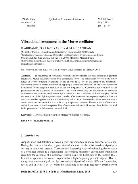
PRAMANA c○ <strong>Indian</strong> <strong>Academy</strong> <strong>of</strong> Sciences Vol. 81, No. 1<br />
— journal <strong>of</strong> July 2013<br />
physics pp. 127–141<br />
<strong>Vibrational</strong> <strong>resonance</strong> <strong>in</strong> <strong>the</strong> <strong>Morse</strong> <strong>oscillator</strong><br />
K ABIRAMI 1 , S RAJASEKAR 1,∗ and M A F SANJUAN 2<br />
1 School <strong>of</strong> Physics, Bharathidasan University, Tiruchirapalli 620 024, India<br />
2 Nonl<strong>in</strong>ear Dynamics, Chaos and Complex Systems Group, Departamento de Física,<br />
Universidad Rey Juan Carlos, Tulipán s/n, 28933 Móstoles, Madrid, Spa<strong>in</strong><br />
∗ Correspond<strong>in</strong>g author. E-mail: rajasekar@cnld.bdu.ac.<strong>in</strong>; nk.abirami@gmail.com;<br />
miguel.sanjuan@urjc.es<br />
MS received 21 June 2012; revised 8 February 2013; accepted 26 February 2013<br />
Abstract. The occurrence <strong>of</strong> vibrational <strong>resonance</strong> is <strong>in</strong>vestigated <strong>in</strong> both classical and quantum<br />
mechanical <strong>Morse</strong> <strong>oscillator</strong>s driven by a biharmonic force. The biharmonic force consists <strong>of</strong> two<br />
forces <strong>of</strong> widely different frequencies ω and with ≫ ω. In <strong>the</strong> damped and biharmonically<br />
driven classical <strong>Morse</strong> <strong>oscillator</strong>, by apply<strong>in</strong>g a <strong>the</strong>oretical approach, an analytical expression<br />
is obta<strong>in</strong>ed for <strong>the</strong> response amplitude at <strong>the</strong> low-frequency ω. Conditions are identified on <strong>the</strong><br />
parameters for <strong>the</strong> occurrence <strong>of</strong> <strong>resonance</strong>. The system shows only one <strong>resonance</strong> and moreover<br />
at <strong>resonance</strong> <strong>the</strong> response amplitude is 1/dω where d is <strong>the</strong> coefficient <strong>of</strong> l<strong>in</strong>ear damp<strong>in</strong>g. When<br />
<strong>the</strong> amplitude <strong>of</strong> <strong>the</strong> high-frequency force is varied after <strong>resonance</strong> <strong>the</strong> response amplitude does not<br />
decay to zero but approaches a nonzero limit<strong>in</strong>g value. It is observed that vibrational <strong>resonance</strong><br />
occurs when <strong>the</strong> s<strong>in</strong>usoidal force is replaced by a square-wave force. The occurrence <strong>of</strong> <strong>resonance</strong><br />
and anti<strong>resonance</strong> <strong>of</strong> transition probability <strong>of</strong> quantum mechanical <strong>Morse</strong> <strong>oscillator</strong> is also reported<br />
<strong>in</strong> <strong>the</strong> presence <strong>of</strong> <strong>the</strong> biharmonic external field.<br />
Keywords. <strong>Morse</strong> <strong>oscillator</strong>; biharmonic force; vibrational <strong>resonance</strong>.<br />
PACS Nos<br />
46.40.Ff; 05.45.−a<br />
1. Introduction<br />
Amplification and detection <strong>of</strong> weak signals are important <strong>in</strong> many branches <strong>of</strong> science.<br />
Dur<strong>in</strong>g <strong>the</strong> past two decades, a great deal <strong>of</strong> attention has been focussed on signal process<strong>in</strong>g<br />
<strong>in</strong> nonl<strong>in</strong>ear systems. There are few <strong>in</strong>terest<strong>in</strong>g ways <strong>of</strong> enhanc<strong>in</strong>g <strong>the</strong> response<br />
<strong>of</strong> a nonl<strong>in</strong>ear system to a weak signal. In stochastic <strong>resonance</strong>, an optimum weak noise<br />
amplifies <strong>the</strong> response <strong>of</strong> a nonl<strong>in</strong>ear system us<strong>in</strong>g <strong>the</strong> bistability <strong>of</strong> <strong>the</strong> system [1,2].<br />
In ano<strong>the</strong>r approach <strong>the</strong> noise is replaced by a high-frequency periodic signal. That is,<br />
<strong>the</strong> system is essentially driven by two periodic signals <strong>of</strong> widely different frequencies,<br />
say, ω and with ≫ ω. When <strong>the</strong> amplitude <strong>of</strong> <strong>the</strong> high-frequency external force<br />
DOI: 10.1007/s12043-013-0546-z; ePublication: 8 June 2013 127
K Abirami, S Rajasekar and M A F Sanjuan<br />
is varied, <strong>the</strong> oscillation amplitude <strong>of</strong> <strong>the</strong> system at <strong>the</strong> low-frequency ω exhibits <strong>resonance</strong>.<br />
This high-frequency force-<strong>in</strong>duced <strong>resonance</strong> is termed as vibrational <strong>resonance</strong><br />
[3–5]. One-way or unidirectional coupl<strong>in</strong>g can also improve <strong>the</strong> performance <strong>of</strong> coupled<br />
systems [6–8]. The same phenomenon can also be observed when besides a noise or a<br />
high-frequency signal, a chaotic signal is used to perturb <strong>the</strong> system [9,10].<br />
The study <strong>of</strong> vibrational <strong>resonance</strong> <strong>in</strong> <strong>the</strong> presence <strong>of</strong> a biharmonic force has received<br />
considerable attention <strong>in</strong> recent years after <strong>the</strong> sem<strong>in</strong>al paper by Landa and McCl<strong>in</strong>tock<br />
[3]. The occurrence <strong>of</strong> vibrational <strong>resonance</strong> has been analysed <strong>in</strong> systems with monostable<br />
[11], bistable [3–5], spatially periodic states [12], excitable systems [13,14], coupled<br />
<strong>oscillator</strong>s [15] and small-world networks [14,16,17]. Experimental evidence <strong>of</strong> vibrational<br />
<strong>resonance</strong> <strong>in</strong> vertical cavity laser system [18–20] and <strong>in</strong> an electronic circuit [21]<br />
has also been reported. Frequency-<strong>resonance</strong>-enhanced vibrational [22] and undamped<br />
signal propagation <strong>in</strong> one-way coupled <strong>oscillator</strong>s [23] and maps [24] assisted by<br />
biharmonic force are found to occur as well.<br />
It is important to <strong>in</strong>vestigate <strong>the</strong> vibrational <strong>resonance</strong> <strong>in</strong> different k<strong>in</strong>ds <strong>of</strong> systems and<br />
br<strong>in</strong>g out its various features and <strong>the</strong> <strong>in</strong>fluence <strong>of</strong> characteristics <strong>of</strong> <strong>the</strong> potential <strong>of</strong> <strong>the</strong><br />
system on it. In this connection we po<strong>in</strong>t out that (i) one or more <strong>resonance</strong>s <strong>in</strong> monostable<br />
systems [11], (ii) a sequence <strong>of</strong> <strong>resonance</strong> peaks <strong>in</strong> a spatially periodic potential<br />
system [12], (iii) additional <strong>resonance</strong>s due to asymmetry <strong>in</strong> <strong>the</strong> potential [25], periodic<br />
and quasiperiodic occurrence <strong>of</strong> <strong>resonance</strong> peaks <strong>in</strong> time-delayed feedback systems<br />
[26–29] and large amplitude <strong>of</strong> vibrational <strong>resonance</strong> at <strong>the</strong> dynamic bifurcation po<strong>in</strong>t<br />
[30] have been reported.<br />
Motivated by some <strong>of</strong> <strong>the</strong> previous results, <strong>in</strong> <strong>the</strong> present paper we report our <strong>in</strong>vestigation<br />
on <strong>the</strong> vibrational <strong>resonance</strong> <strong>in</strong> <strong>the</strong> <strong>Morse</strong> <strong>oscillator</strong>. The potential <strong>of</strong> <strong>the</strong> <strong>Morse</strong><br />
<strong>oscillator</strong> is<br />
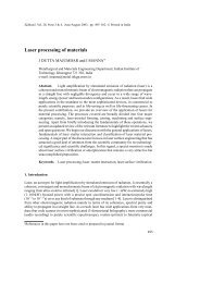
V (x) = 1 2 βe−x (e −x − 2), (1)<br />
where β is a constant parameter represent<strong>in</strong>g <strong>the</strong> dissociation energy. Figure 1 depicts<br />
<strong>the</strong> form <strong>of</strong> <strong>the</strong> potential for a few values <strong>of</strong> β. The potential is nonpolynomial and<br />
V (x) →∞as x →−∞while it becomes zero when x →∞. It has one local m<strong>in</strong>imum<br />
1<br />
0<br />
-1<br />
-1<br />
0<br />
1<br />
2<br />
3<br />
4<br />
5<br />
Figure 1. The shape <strong>of</strong> <strong>the</strong> <strong>Morse</strong> potential for three values <strong>of</strong> β.<br />
128 Pramana – J. Phys., Vol. 81, No. 1, July 2013
<strong>Vibrational</strong> <strong>resonance</strong> <strong>in</strong> <strong>the</strong> <strong>Morse</strong> <strong>oscillator</strong><br />
at x = 0 and <strong>the</strong> depth <strong>of</strong> <strong>the</strong> potential is β/2. The <strong>Morse</strong> <strong>oscillator</strong> was <strong>in</strong>troduced as a<br />
useful model for <strong>the</strong> <strong>in</strong>teratomic potential and fitt<strong>in</strong>g <strong>the</strong> vibrational spectra <strong>of</strong> diatomic<br />
molecules. It was also used to describe <strong>the</strong> photodissociation <strong>of</strong> molecules, multiphoton<br />
excitation <strong>of</strong> <strong>the</strong> diatomic molecules <strong>in</strong> a dense medium or <strong>in</strong> a gaseous cell under high<br />
pressure and pump<strong>in</strong>g <strong>of</strong> a local model <strong>of</strong> a polyatomic molecule by an <strong>in</strong>frared laser<br />
[31–34]. The existence and bifurcations <strong>of</strong> periodic orbits have been studied <strong>in</strong> detail <strong>in</strong><br />
[35,36].<br />
The equation <strong>of</strong> motion <strong>of</strong> <strong>the</strong> damped and biharmonically-driven classical <strong>Morse</strong><br />
<strong>oscillator</strong> is given by<br />
ẍ + dẋ + βe −x (1 − e −x ) = f cos ωt + g cos t, ≫ ω. (2)<br />
Because <strong>of</strong> <strong>the</strong> difference <strong>in</strong> time-scales <strong>of</strong> <strong>the</strong> two periodic forces, <strong>the</strong> motion <strong>of</strong> system<br />
(2) conta<strong>in</strong>s both a slow component X (t) with period T = 2π/ω and a fast vary<strong>in</strong>g component<br />
ψ(t, τ= t) with period 2π/. That is, we assumed that x(t) = X (t)+ψ(t,τ).<br />
When <strong>the</strong> amplitude g or frequency is varied, <strong>the</strong> response <strong>of</strong> system (2) at <strong>the</strong> frequency<br />
ω can exhibit <strong>resonance</strong> at a particular value <strong>of</strong> <strong>the</strong> control parameter g or . To<br />
analyse this <strong>resonance</strong> phenomenon and <strong>the</strong> <strong>in</strong>fluence <strong>of</strong> <strong>the</strong> shape <strong>of</strong> <strong>the</strong> potential on <strong>the</strong><br />
<strong>resonance</strong> we obta<strong>in</strong>ed an equation <strong>of</strong> motion for <strong>the</strong> slow variable by apply<strong>in</strong>g a perturbation<br />
<strong>the</strong>ory. From <strong>the</strong> solution <strong>of</strong> <strong>the</strong> l<strong>in</strong>earized version <strong>of</strong> <strong>the</strong> equation <strong>of</strong> motion about its<br />
equilibrium po<strong>in</strong>t, we found <strong>the</strong> analytical expression for <strong>the</strong> response amplitude Q which<br />
is <strong>the</strong> ratio <strong>of</strong> <strong>the</strong> amplitude <strong>of</strong> oscillation <strong>of</strong> <strong>the</strong> output <strong>of</strong> <strong>the</strong> system at <strong>the</strong> frequency ω<br />
and <strong>the</strong> amplitude f <strong>of</strong> <strong>the</strong> <strong>in</strong>put signal. From <strong>the</strong> expression <strong>of</strong> Q, we extracted various<br />
features <strong>of</strong> vibrational <strong>resonance</strong> <strong>in</strong> <strong>the</strong> <strong>Morse</strong> <strong>oscillator</strong>. Particularly, we determ<strong>in</strong>ed<br />
<strong>the</strong> value <strong>of</strong> g at which <strong>resonance</strong> occurs, <strong>the</strong> maximum value <strong>of</strong> Q at <strong>resonance</strong> and<br />
<strong>the</strong> limit<strong>in</strong>g value <strong>of</strong> Q. We confirmed all <strong>the</strong> <strong>the</strong>oretical predictions through numerical<br />
simulation. The <strong>the</strong>oretical treatment used for <strong>the</strong> analysis <strong>of</strong> <strong>the</strong> vibrational <strong>resonance</strong><br />
with <strong>the</strong> periodic force f cos ωt + g cos t can be applied for o<strong>the</strong>r types <strong>of</strong> biharmonic<br />
forces. In particular, we illustrated this for a square-wave form <strong>of</strong> low-frequency and<br />
high-frequency forces. Next, we considered <strong>the</strong> quantum mechanical <strong>Morse</strong> <strong>oscillator</strong><br />
subjected to <strong>the</strong> biharmonic external field. Apply<strong>in</strong>g a perturbation <strong>the</strong>ory we obta<strong>in</strong>ed an<br />
analytical expression for <strong>the</strong> first-order transition probability P fi for a transition from an<br />
ith quantum state to an f th quantum state <strong>in</strong> time T caused by <strong>the</strong> applied external field.<br />
We analysed <strong>the</strong> <strong>in</strong>fluence <strong>of</strong> high-frequency field on P fi and showed <strong>the</strong> occurrence <strong>of</strong><br />
<strong>resonance</strong> and anti<strong>resonance</strong>.<br />
2. Classical <strong>Morse</strong> <strong>oscillator</strong><br />
In this section <strong>the</strong> classical <strong>Morse</strong> <strong>oscillator</strong> described by <strong>the</strong> equation <strong>of</strong> motion (2) is<br />
considered and <strong>the</strong> occurrence <strong>of</strong> vibrational <strong>resonance</strong> is analysed.<br />
2.1 Theoretical approach<br />
To f<strong>in</strong>d an approximate solution <strong>of</strong> eq. (2), we used <strong>the</strong> method <strong>of</strong> separation <strong>of</strong> variables<br />
by assum<strong>in</strong>g x = X (t) + ψ(t, τ = t), where X and ψ are slow and fast variables<br />
Pramana – J. Phys., Vol. 81, No. 1, July 2013 129
K Abirami, S Rajasekar and M A F Sanjuan<br />
respectively. Substitut<strong>in</strong>g x = X + ψ <strong>in</strong> eq. (2) and add<strong>in</strong>g and subtract<strong>in</strong>g <strong>the</strong> terms<br />
β〈e −ψ 〉e −x and β〈e −2ψ 〉e −2x where 〈u〉 =(1/2π) ∫ 2π<br />
0<br />
u dτ, τ = t we obta<strong>in</strong><br />
Ẍ + d Ẋ + βe −X (〈e −ψ 〉−〈e −2ψ 〉e −X ) = f cos ωt, (3)<br />
¨ψ + d ˙ψ + βe −X (e −ψ −〈e −ψ 〉) − βe −2X (e −2ψ −〈e −2ψ 〉) = g cos t. (4)<br />
As ψ is a rapidly chang<strong>in</strong>g variable with fast time τ we approximated eq. (4) as ¨ψ =<br />
g cos t. The solution <strong>of</strong> this equation is ψ = μ cos t where μ = g/ 2 . This solution<br />
gives<br />
∫ 2π<br />
〈e −ψ 〉= 1 e μ cos τ dτ = I 0 (μ),<br />
(5a)<br />
2 0<br />
〈e −2ψ 〉=I 0 (2μ), (5b)<br />
where I 0 (z) is <strong>the</strong> zeroth-order modified Bessel function [37]. Now, eq. (3) becomes<br />
Ẍ + d Ẋ + βe −X (I 0 (μ) − I 0 (2μ)e −X ) = f cos ωt. (6)<br />
Equation (6) can be treated as <strong>the</strong> equation <strong>of</strong> motion <strong>of</strong> a particle experienc<strong>in</strong>g <strong>the</strong><br />
external periodic force f cos ωt and l<strong>in</strong>ear friction force <strong>in</strong> <strong>the</strong> effective potential<br />
V eff = 1 2 βe−X [I 0 (2μ)e −X − 2I 0 (μ)]. (7)<br />
In addition to <strong>the</strong> parameter β, <strong>the</strong> effective potential depends on <strong>the</strong> parameters g and<br />
. The dependence <strong>of</strong> V eff on g and is <strong>in</strong> <strong>the</strong> form <strong>of</strong> a zeroth-order modified Bessel<br />
function.<br />
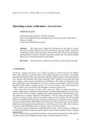
Figure 2a depicts <strong>the</strong> variation <strong>of</strong> I 0 (μ) and I 0 (2μ) with g for = 10. As g<br />
<strong>in</strong>creases from zero, <strong>the</strong> values <strong>of</strong> I 0 (μ) and I 0 (2μ) <strong>in</strong>crease from <strong>the</strong> value 1. I 0 (2μ)<br />
<strong>in</strong>creases more rapidly than I 0 (μ) with g. Figure 2b shows <strong>the</strong> change <strong>in</strong> <strong>the</strong> shape <strong>of</strong><br />
<strong>the</strong> effective potential with g. The location <strong>of</strong> <strong>the</strong> m<strong>in</strong>imum <strong>of</strong> <strong>the</strong> potential V eff (X) or <strong>the</strong><br />
X-component <strong>of</strong> <strong>the</strong> equilibrium po<strong>in</strong>t <strong>of</strong> <strong>the</strong> system (6) <strong>in</strong> <strong>the</strong> absence <strong>of</strong> periodic driv<strong>in</strong>g<br />
force is given by<br />
( )<br />
X ∗ I0 (μ)<br />
=−ln . (8)<br />
I 0 (2μ)<br />
10<br />
1<br />
5<br />
0<br />
(a)<br />
0<br />
0<br />
200<br />
400<br />
-1<br />
-1<br />
(b)<br />
0<br />
1<br />
2<br />
3<br />
4<br />
5<br />
Figure 2. (a) Dependence <strong>of</strong> zeroth-order modified Bessel function with <strong>the</strong> control<br />
parameter g when = 10 and μ = g/ 2 . (b) Plot <strong>of</strong> <strong>the</strong> effective potential V eff<br />
given by eq. (7) for three values <strong>of</strong> g with β = 2and = 10.<br />
130 Pramana – J. Phys., Vol. 81, No. 1, July 2013
<strong>Vibrational</strong> <strong>resonance</strong> <strong>in</strong> <strong>the</strong> <strong>Morse</strong> <strong>oscillator</strong><br />
As I 0 (2μ) > I 0 (μ), X ∗ is always greater than 0 and it moves away from <strong>the</strong> orig<strong>in</strong> as<br />
g <strong>in</strong>creases. Consequently, <strong>the</strong> depth V eff =|V eff (X ∗ )|=β I 2 0 (μ)/2I 0(2μ) decreases<br />
with <strong>in</strong>crease <strong>in</strong> g and <strong>the</strong> potential V eff becomes more and more flat. Later, we po<strong>in</strong>ted<br />
out an important consequence <strong>of</strong> this on <strong>the</strong> response amplitude Q.<br />
A slow oscillation takes place about X ∗ . Therefore, for convenience, a change <strong>of</strong> variable<br />
Y = X − X ∗ is <strong>in</strong>troduced so that slow oscillation occurs around Y ∗ = 0. In terms<br />
<strong>of</strong> Y , eq. (6) becomes<br />
Ÿ + dẎ + ω 2 r e−Y (1 − e −Y ) = f cos ωt,<br />
(9a)<br />
where<br />
ωr 2 = β I 0 2(μ)<br />
I 0 (2μ) .<br />
(9b)<br />
For | f |≪1 it is reasonable to assume that <strong>the</strong> amplitude <strong>of</strong> Y is small so that series<br />
expansions for e −Y and e −2Y can be written and nonl<strong>in</strong>ear terms <strong>in</strong> Y can be neglected.<br />
This results <strong>in</strong> <strong>the</strong> l<strong>in</strong>ear equation<br />
Ÿ + dẎ + ωr 2 Y = f cos ωt. (10)<br />
ω r is <strong>the</strong> resonant frequency <strong>of</strong> oscillation <strong>of</strong> <strong>the</strong> slow motion. In <strong>the</strong> long time limit, <strong>the</strong><br />
solution <strong>of</strong> eq. (10) isY = Qf cos(ωt + φ) where<br />
Q = √ 1 , S = (ωr 2 − ω2 ) 2 + d 2 ω 2 , (11a)<br />
S<br />
and<br />
φ = tan −1 (<br />
dω<br />
ω 2 − ω 2 r<br />
)<br />
, (11b)<br />
where Q is <strong>the</strong> response amplitude <strong>of</strong> system (2) at <strong>the</strong> low-frequency ω <strong>of</strong> <strong>the</strong> <strong>in</strong>put<br />
signal.<br />
2.2 Analysis <strong>of</strong> <strong>the</strong> vibrational <strong>resonance</strong><br />
In order to verify <strong>the</strong> <strong>the</strong>oretical predictions to be obta<strong>in</strong>ed from <strong>the</strong> analysis <strong>of</strong> Q given<br />
by √ eq. (11a), Q is calculated from <strong>the</strong> numerical solution <strong>of</strong> eq. (2). The formula Q =<br />
Q<br />
2 s + Q 2 c /f is used where [3,5,13]<br />
Q s = 2 ∫ nT<br />
x(t) s<strong>in</strong> ωt dt,<br />
(12a)<br />
nT 0<br />
Q c = 2 ∫ nT<br />
x(t) cos ωt dt,<br />
(12b)<br />
nT 0<br />
with T = 2π/ω and n is big enough, say 500.<br />
The value <strong>of</strong> a control parameter at which <strong>resonance</strong> occurs (Q becomes maximum)<br />
corresponds to <strong>the</strong> m<strong>in</strong>imum <strong>of</strong> <strong>the</strong> function S given by eq. (11a). The follow<strong>in</strong>g are <strong>the</strong><br />
key results <strong>of</strong> analysis <strong>of</strong> <strong>the</strong> <strong>the</strong>oretical expression <strong>of</strong> <strong>the</strong> response amplitude Q.<br />
Pramana – J. Phys., Vol. 81, No. 1, July 2013 131
K Abirami, S Rajasekar and M A F Sanjuan<br />
• For a fixed value <strong>of</strong> g when ω is varied, <strong>resonance</strong> occurs when ω = ω VR where ω VR<br />
is given by (obta<strong>in</strong>ed from dS/dω = 0)<br />
√<br />
ω VR = ωr 2 − d2<br />
2 , ω2 r > d2<br />
2 . (13)<br />
• When g is varied <strong>the</strong> condition for <strong>resonance</strong> is dS/dg = 4ω r ω rg (ωr 2 − ω 2 ) = 0.<br />
Because I 0 is always >0 and <strong>in</strong>creases monotonically with g we have ω r ̸= 0<br />
and ω rg = dω r /dg ̸= 0 and hence <strong>the</strong> <strong>resonance</strong> condition is ωr 2 = ω 2 , that is,<br />
β I0 2(g/2 )/I 0 (2g/ 2 ) = ω 2 . Resonance occurs whenever <strong>the</strong> resonant frequency<br />
ω r matches with <strong>the</strong> low-frequency ω <strong>of</strong> <strong>the</strong> periodic force.<br />
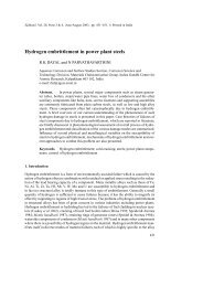
• Figures 3a and b show <strong>the</strong> variation <strong>of</strong> <strong>the</strong> response amplitude Q and ωr 2 respectively<br />
with g for three fixed values <strong>of</strong> β and d = 0.5, f = 0.1, ω= 1 and = 10. The<br />
<strong>the</strong>oretical value <strong>of</strong> Q is <strong>in</strong> very good agreement with Q obta<strong>in</strong>ed from <strong>the</strong> numerical<br />
solution <strong>of</strong> eq. (2). In figure 3a, for both β = 2 and 1.5, as g <strong>in</strong>creases from zero<br />
<strong>the</strong> value <strong>of</strong> Q <strong>in</strong>creases monotonically, it reaches a maximum at g = g VR and <strong>the</strong>n<br />
decreases. For β = 2, <strong>the</strong> <strong>the</strong>oretical and numerical values <strong>of</strong> g VR are 176 and 173<br />
respectively. In figure 3b for both β = 2 and 1.5 atg = g VR (<strong>in</strong>dicated by solid<br />
circles), ωr 2 = ω2 .<br />
• At g = 0, I 0 (μ) = I 0 (2μ) = 1 and ωr 2(g = 0) = β. As g <strong>in</strong>creases, I 0(μ) and<br />
I 0 (2μ) <strong>in</strong>crease rapidly with I 0 (2μ) grow<strong>in</strong>g faster than I 0 (μ) as shown <strong>in</strong> figure 2a.<br />
Consequently, ωr 2 decreases rapidly from <strong>the</strong> value <strong>of</strong> β for a while and <strong>the</strong>n decays<br />
to zero slowly. The maximum value <strong>of</strong> ωr 2 is β and this happens at g = 0. For β<<br />
ω 2 , ωr 2 is always less than ω2 , that is, ωr 2 ̸= ω2 for g > 0 imply<strong>in</strong>g no <strong>resonance</strong>. This<br />
is shown <strong>in</strong> figure 3a forβ = 0.5 and ω = 1forwhichQ decreases cont<strong>in</strong>uously<br />
with g.<br />
• Resonance is possible only for β>ω 2 . In this case, as g <strong>in</strong>creases from zero, ωr<br />
2<br />
decreases and becomes ω 2 at only one value. Hence, <strong>the</strong>re is only one <strong>resonance</strong>.<br />
2<br />
2 1<br />
2<br />
2<br />
1<br />
1<br />
(a)<br />
1<br />
0<br />
3<br />
500<br />
1000<br />
(b)<br />
3<br />
0<br />
0<br />
500<br />
1000<br />
Figure 3. (a) Response amplitude Q vs. <strong>the</strong> control parameter g for <strong>the</strong> <strong>Morse</strong> <strong>oscillator</strong><br />
for three values <strong>of</strong> β. The values <strong>of</strong> <strong>the</strong> parameters are d = 0.5, f = 0.1, ω= 1<br />
and = 10. The values <strong>of</strong> β for <strong>the</strong> curves 1, 2 and 3 are 2, 1.5and0.5 respectively.<br />
The cont<strong>in</strong>uous curve and solid circles represent <strong>the</strong>oretically and numerically computed<br />
values <strong>of</strong> Q respectively. The horizontal dashed l<strong>in</strong>e denotes <strong>the</strong> limit<strong>in</strong>g value<br />
<strong>of</strong> Q, Q L (g →∞). (b) Dependence <strong>of</strong> ωr 2 with g for <strong>the</strong> three values <strong>of</strong> β used <strong>in</strong><br />
figure 3a. The solid circles on <strong>the</strong> g axis denote <strong>the</strong> values <strong>of</strong> g at which <strong>resonance</strong><br />
occurs.<br />
132 Pramana – J. Phys., Vol. 81, No. 1, July 2013
<strong>Vibrational</strong> <strong>resonance</strong> <strong>in</strong> <strong>the</strong> <strong>Morse</strong> <strong>oscillator</strong><br />
2<br />
1<br />
2<br />
1<br />
0<br />
0<br />
250<br />
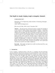
Figure 4. Three-dimensional plot <strong>of</strong> <strong>the</strong> <strong>the</strong>oretically computed response amplitude<br />
Q as a function <strong>of</strong> β and g.<br />
500<br />
This is shown <strong>in</strong> figure 3a forβ = 1.5 and 2 with ω = 1. Figure 4 presents <strong>the</strong><br />
dependence <strong>of</strong> Q on β and g for ω = 1. Resonance is seen only for β>ω 2 (= 1).<br />
• At <strong>resonance</strong> ωr 2 = ω 2 and hence Q max = 1/dω and it depends only on d and ω.<br />
The response amplitude at <strong>resonance</strong> is <strong>in</strong>dependent <strong>of</strong> <strong>the</strong> parameters β, g and .<br />
• An analytical expression for g VR (at which Q becomes maximum) is difficult to<br />
obta<strong>in</strong> because ωr 2 is a complicated function <strong>of</strong> g. However, g VR can be calculated<br />
from <strong>the</strong> <strong>resonance</strong> curve. It depends on , ω and β and <strong>in</strong>dependent <strong>of</strong> d and f .<br />
Q decreases with <strong>in</strong>crease <strong>in</strong> <strong>the</strong> value <strong>of</strong> d. In figure 5 we plot <strong>the</strong> <strong>the</strong>oretically<br />
predicted g VR and numerically computed g VR vs. <strong>the</strong> parameter β for a few fixed<br />
values <strong>of</strong> ω. g VR <strong>in</strong>creases with <strong>in</strong>crease <strong>in</strong> <strong>the</strong> value <strong>of</strong> β.<br />
• For very large values <strong>of</strong> g, ωr 2 → 0 and Q approaches <strong>the</strong> limit<strong>in</strong>g value Q L given by<br />
1<br />
Q L (g →∞) =<br />
ω √ ω 2 + d . (14)<br />
2<br />
That is, Q does not decay to zero but approaches <strong>the</strong> above limit<strong>in</strong>g value (see figure<br />
3a). This limit<strong>in</strong>g value depends only on <strong>the</strong> parameters ω and d (note that<br />
Q max = 1/dω). The po<strong>in</strong>t is that when ωr<br />
2 → 0, eq. (9) becomes <strong>the</strong> damped free<br />
particle driven by <strong>the</strong> periodic force whose solution is<br />
Y (t) = Q L f cos(ωt + ), = tan −1 (d/ω). (15)<br />
250<br />
150<br />
50<br />
0<br />
1<br />
2<br />
Figure 5. Variation <strong>of</strong> <strong>the</strong>oretically predicted (cont<strong>in</strong>uous curve) and numerically<br />
computed (solid circles) g VR with <strong>the</strong> parameter β for a few fixed values <strong>of</strong> <strong>the</strong><br />
parameter ω. The value <strong>of</strong> is 10ω.<br />
Pramana – J. Phys., Vol. 81, No. 1, July 2013 133
K Abirami, S Rajasekar and M A F Sanjuan<br />
For <strong>the</strong> Duff<strong>in</strong>g and qu<strong>in</strong>tic <strong>oscillator</strong>s [3,5,11,25] V (x) (as well as <strong>the</strong> effective<br />
potential) →∞as x →±∞. In this case <strong>the</strong> resonant frequency diverges after a<br />
few oscillations and thus Q decays to zero for large values <strong>of</strong> g.<br />
3. Resonance with a square-wave signal<br />
In this section we show that vibrational <strong>resonance</strong> can be realized <strong>in</strong> <strong>the</strong> <strong>Morse</strong> <strong>oscillator</strong><br />
when <strong>the</strong> external signal is a square-wave and <strong>the</strong> <strong>the</strong>oretical analysis employed <strong>in</strong> <strong>the</strong><br />
previous section for s<strong>in</strong>usoidal force can be applied to this case also.<br />
In system (2), <strong>in</strong> place <strong>of</strong> F 1 = f cos ωt + g cos t, we consider three o<strong>the</strong>r forms <strong>of</strong><br />
external force given by<br />
F 2 (t) = f cos ωt + g sgn(cos t), (16)<br />
F 3 (t) = f sgn(cos ωt) + g cos t, (17)<br />
F 4 (t) = f sgn(cos ωt) + g sgn(cos t), (18)<br />
where sgn|u| denotes sign <strong>of</strong> u. In <strong>the</strong> <strong>the</strong>oretical analysis we use a Fourier series expansion<br />
for <strong>the</strong> square-wave signal. For <strong>the</strong> <strong>Morse</strong> <strong>oscillator</strong> driven by <strong>the</strong> periodic force<br />
F 2 (t) <strong>the</strong> solution <strong>of</strong> slow motion is Y 2 = Q 2 f cos(ωt + φ 2 ) where<br />
Q 2 =<br />
1<br />
√(ω 2 r,2 − ω2 ) 2 + d 2 ω 2 , (19a)<br />
where<br />
∫ 2π<br />
ωr,2 2 = βU 2 (μ)<br />
U(2μ) , U(μ) = 1<br />
2π 0<br />
e −ψ 2<br />
dτ,<br />
(19b)<br />
ψ 2 = 4μ ∞∑ (−1) n+1 cos(2n + 1)τ<br />
.<br />
π (2n + 1) 3 n=0<br />
(19c)<br />
For <strong>the</strong> system driven by <strong>the</strong> force F 3 , <strong>the</strong> solution Y 3 is<br />
Y 3 = 4 f ∞∑ (−1) n<br />
cos[(2n + 1)ωt + φ 3 ]<br />
π (2n + 1) [(ω 2 n=0<br />
r,3 − (2n + 1)2 ω 2 ) 2 + (2n + 1) 2 d 2 ω 2 ] , 1/2 (20a)<br />
where<br />
ωr,3 2 = β I 0 2(μ)<br />
I 0 (2μ) .<br />
(20b)<br />
The solution Y 3 has frequencies ω and odd <strong>in</strong>teger multiples <strong>of</strong> it. The response amplitude<br />
Q 3 correspond<strong>in</strong>g to <strong>the</strong> fundamental frequency ω is<br />
Q 3 = 4 1<br />
.<br />
π<br />
√(ωr,3 2 − ω2 ) 2 + d 2 ω 2 (21)<br />
When <strong>the</strong> biharmonic force is chosen as F 4 given by eq. (18) <strong>the</strong>n <strong>the</strong> expression for <strong>the</strong><br />
solution Y 4 is <strong>the</strong> same as Y 3 except that now ωr,3 2 is replaced by ω2 r,4 where<br />
ωr,4 2 = βU 2 (μ)<br />
U(2μ) . (22)<br />
134 Pramana – J. Phys., Vol. 81, No. 1, July 2013
<strong>Vibrational</strong> <strong>resonance</strong> <strong>in</strong> <strong>the</strong> <strong>Morse</strong> <strong>oscillator</strong><br />
Then<br />
Q 4 = 4 π<br />
1<br />
√(ω 2 r,4 − ω2 ) 2 + d 2 ω 2 . (23)<br />
Figure 6 shows both <strong>the</strong>oretically determ<strong>in</strong>ed Q and numerically computed Q vs. g<br />
with different <strong>in</strong>put signals where d = 0.5, β= 2, f = 0.1, ω= 1 and = 10. In<br />
this figure, apart from <strong>the</strong> close agreement <strong>of</strong> <strong>the</strong>oretical Q with numerical Q, we notice<br />
that Q 1,max = Q 2,max , Q 3,max = Q 4,max , Q 1,L = Q 2,L (limit<strong>in</strong>g values <strong>of</strong> Q <strong>in</strong> <strong>the</strong> limit<br />
<strong>of</strong> g → ∞) and Q 3,L = Q 4,L . These results can be accounted from <strong>the</strong> <strong>the</strong>oretical<br />
expressions <strong>of</strong> Q i . The <strong>resonance</strong> condition ωr,i 2 = ω 2 , i = 1, 2, 3, 4 <strong>in</strong> <strong>the</strong> expression<br />
<strong>of</strong> Q i gives<br />
Q 1,max = Q 2,max = 1<br />
dω ,<br />
(24a)<br />
Q 3,max = Q 4,max = 4<br />
πdω = 4 π Q 1,max,<br />
(24b)<br />
that is, Q 3,max and Q 4,max are 4/π ≈ 1.27324 times <strong>of</strong> Q 1,max . For <strong>the</strong> parametric values<br />
used <strong>in</strong> our analysis, Q 1,max = 2 and hence Q 3,max and Q 4,max are 2.54648 as is <strong>the</strong> case<br />
<strong>in</strong> figure 6. For sufficiently large values <strong>of</strong> g, ωr,i 2 ≈ 0 and hence<br />
1<br />
Q 1,L = Q 2,L =<br />
ω √ ω 2 + d , Q 2 3,L = Q 4,L = 4 π Q 1,L. (25)<br />
Fur<strong>the</strong>rmore, because <strong>of</strong> ωr,1 2 = ω2 r,3 and ω2 r,2 = ω2 r,4<br />
it is found that<br />
Q 3 = 4 π Q 1, Q 4 = 4 π Q 2. (26)<br />
That is, <strong>the</strong> response amplitude at frequency ω when <strong>the</strong> <strong>in</strong>put signal is a square-wave<br />
with fundamental frequency be<strong>in</strong>g ω is 4/π times that <strong>of</strong> <strong>the</strong> signal f cos ωt. Numerical<br />
results <strong>in</strong> figure 6 confirms all <strong>the</strong> above <strong>the</strong>oretical predictions.<br />
2.5<br />
2<br />
1.5<br />
4<br />
2<br />
3<br />
1<br />
1<br />
0<br />
300<br />
600<br />
Figure 6. Variation <strong>of</strong> <strong>the</strong> response amplitude Q with g for four different types<br />
<strong>of</strong> biharmonic forces. The cont<strong>in</strong>uous curves and <strong>the</strong> solid circles represent <strong>the</strong>oretically<br />
calculated Q and numerically calculated Q respectively. The biharmonic<br />
forces correspond<strong>in</strong>g to <strong>the</strong> curves and solid circles marked as 1, 2, 3 and 4 are<br />
f cos ωt + g cos t, F 2 , F 3 and F 4 respectively.<br />
Pramana – J. Phys., Vol. 81, No. 1, July 2013 135
K Abirami, S Rajasekar and M A F Sanjuan<br />
Our analysis shows that <strong>the</strong> form <strong>of</strong> <strong>the</strong> low- and high-frequency forces need not be<br />
identical. For any arbitrary force conta<strong>in</strong><strong>in</strong>g a component with frequency ω, enhancement<br />
<strong>of</strong> <strong>the</strong> amplitude <strong>of</strong> <strong>the</strong> output signal at frequency ω can be achieved by us<strong>in</strong>g ano<strong>the</strong>r<br />
arbitrary force conta<strong>in</strong><strong>in</strong>g a frequency ≫ ω. When <strong>the</strong> force <strong>in</strong>volved is simple periodic<br />
function <strong>of</strong> t, <strong>the</strong>n <strong>the</strong> <strong>the</strong>oretical analysis <strong>of</strong> vibrational <strong>resonance</strong> is very much feasible.<br />
4. Quantum mechanical <strong>Morse</strong> <strong>oscillator</strong><br />
In <strong>the</strong> previous two sections, our analysis was focussed on vibrational <strong>resonance</strong> <strong>in</strong><br />
<strong>the</strong> classical <strong>Morse</strong> <strong>oscillator</strong>. In <strong>the</strong> present section we are concerned with <strong>the</strong> quantum<br />
mechanical <strong>Morse</strong> <strong>oscillator</strong> <strong>in</strong> <strong>the</strong> presence <strong>of</strong> biharmonic external field W (t) =<br />
F cos ωt + g cos t with ≫ ω. When a quantum mechanical system is subjected to a<br />
time-dependent external field, <strong>the</strong> system undergoes transition between <strong>the</strong> energy eigenstates.<br />
Therefore, we are <strong>in</strong>terested <strong>in</strong> know<strong>in</strong>g <strong>the</strong> probability <strong>of</strong> f<strong>in</strong>d<strong>in</strong>g <strong>the</strong> system <strong>in</strong> an<br />
f th state at time t.<br />
The unperturbed Hamiltonian <strong>of</strong> <strong>the</strong> system is H 0 = (px 2 /2m) + V (x) where V (x)<br />
is given by eq. (1). The unperturbed system H 0 φ n = E n φ n is exactly solvable and <strong>the</strong><br />
eigenfunctions and energy eigenvalues are given by [38–40]<br />
φ n = N n z λ−n−1/2 e −z/2 L k n (z),<br />
(27a)<br />
where<br />
z = 2λe −x , λ 2 = mβ (<br />
)<br />
¯h 2 , N kn! 1/2<br />
n =<br />
, (27b)<br />
(2λ − n − 1)!<br />
k = 2λ − 2n − 1, L k n (z) = z−k e z d n<br />
n! dz n e−z z n+k<br />
(27c)<br />
and<br />
E n =−¯h 2 (<br />
λ − n − 1 2<br />
, n = 0, 1,... and n
<strong>Vibrational</strong> <strong>resonance</strong> <strong>in</strong> <strong>the</strong> <strong>Morse</strong> <strong>oscillator</strong><br />
2<br />
0<br />
-2<br />
-4<br />
-2<br />
0<br />
2<br />
4<br />
6<br />
8<br />
Figure 7. Bound state energy eigenvalues and eigenfunctions <strong>of</strong> <strong>the</strong> <strong>Morse</strong> <strong>oscillator</strong><br />
for β = 9. The dashed l<strong>in</strong>es are <strong>the</strong> energy eigenvalues. The potential V (x) is also<br />
shown.<br />
The probability <strong>of</strong> f<strong>in</strong>d<strong>in</strong>g <strong>the</strong> system <strong>in</strong> <strong>the</strong> state n is P n (t) =|a n (t)| 2 , ∑ n |a n(t)| 2 = 1.<br />
To determ<strong>in</strong>e a n (t) we apply <strong>the</strong> standard time-dependent perturbation <strong>the</strong>ory [41].<br />
Suppose <strong>the</strong> external field is switched-on at t = 0 and switched-<strong>of</strong>f at t = T , that is,<br />
<strong>the</strong> external field is applied dur<strong>in</strong>g a f<strong>in</strong>ite time <strong>in</strong>terval T . Assume that <strong>the</strong> system is<br />
<strong>in</strong>itially <strong>in</strong> a state i with <strong>the</strong> eigenfunction φ i . Then at t = 0 <strong>the</strong> probability <strong>of</strong> f<strong>in</strong>d<strong>in</strong>g <strong>the</strong><br />
system <strong>in</strong> <strong>the</strong> state i is 1 and <strong>the</strong> probability <strong>of</strong> f<strong>in</strong>d<strong>in</strong>g <strong>the</strong> system <strong>in</strong> <strong>the</strong> o<strong>the</strong>r states is 0:<br />
a n (0) = δ ni . Due to <strong>the</strong> applied field <strong>the</strong> system can make a transition from <strong>the</strong> state i to<br />
an ano<strong>the</strong>r state after <strong>the</strong> time T . Once <strong>the</strong> perturbation is switched-<strong>of</strong>f, <strong>the</strong> system settles<br />
down to a stationary state and this f<strong>in</strong>al state is denoted as f .<br />
To determ<strong>in</strong>e a n (t) we substitute eq. (31), a f = a (0)<br />
f<br />
+ ɛa (1)<br />
f<br />
+··· and equate <strong>the</strong> terms<br />
conta<strong>in</strong><strong>in</strong>g various powers <strong>of</strong> ɛ to 0. Up to first order <strong>in</strong> ɛ, after some algebra, we obta<strong>in</strong><br />
= δ fi and<br />
a (0)<br />
f<br />
where<br />
a (1)<br />
f<br />
(T ) = C fi<br />
2¯h s,<br />
s = F(r 1+ + r 1− ) + g(r 2+ + r 2− ),<br />
(32a)<br />
(32b)<br />
r 1± = 1 − ei(ω fi±ω)T<br />
ω fi ± ω , r 2± = 1 − ei(ω fi±)T<br />
ω fi ± , (32c)<br />
ω fi = (E ∫<br />
f − E i )<br />
∞<br />
, C fi = φ ∗ f<br />
¯h<br />
xφ i dx.<br />
(32d)<br />
−∞<br />
The transition probability for ith state to f th state is given by P fi (T ) =|δ fi +ɛa (1)<br />
f<br />
(T )| 2 .<br />
In a (1)<br />
f<br />
(T ) <strong>the</strong> term s alone depends on <strong>the</strong> parameters F, ω, g and <strong>of</strong> <strong>the</strong> external field<br />
and T . Therefore, we study <strong>the</strong> variation <strong>of</strong> <strong>the</strong> quantity |s| 2 with <strong>the</strong> parameters <strong>of</strong> <strong>the</strong><br />
external field.<br />
We fix β = 9, F = 0.05, T = π and assume that <strong>the</strong> system is <strong>in</strong>itially <strong>in</strong> <strong>the</strong> ground<br />
state (i = 0). Figure 8 shows <strong>the</strong> variation <strong>of</strong> log |s| 2 with ω for g = 0. The firstorder<br />
correction to transition probability displays a sequence <strong>of</strong> <strong>resonance</strong> peaks with<br />
Pramana – J. Phys., Vol. 81, No. 1, July 2013 137
K Abirami, S Rajasekar and M A F Sanjuan<br />
0<br />
-2<br />
-4<br />
-6<br />
-8<br />
0<br />
1<br />
2<br />
3<br />
4<br />
5<br />
6<br />
7<br />
8<br />
Figure 8. log|s| 2 vs. ω for <strong>the</strong> states f = 0, 1 and 2 for β = 9, F = 0.05, g = 0,<br />
T = π and i = 0.<br />
decreas<strong>in</strong>g amplitude. The follow<strong>in</strong>g results are evident from eqs (32b) and (32c) and<br />
figure 8. The quantity s consists <strong>of</strong> only r 1+ and r 1− . We have ω 00 = 0, ω 10 = 2 and<br />
ω 20 = 3. Consequently, for <strong>the</strong> states f = 0, 1 and 2 <strong>the</strong> quantity r 1+ can be neglected<br />
when ω ≈ 0, 2 and 3 respectively because <strong>the</strong> denom<strong>in</strong>ator <strong>in</strong> r 1− is ≈0. Thus, <strong>the</strong> firstorder<br />
transition probability for <strong>the</strong> states f = 0, 1 and 2 becomes maximum at ω = 0, 2<br />
and 3 respectively. For ω ≈ 0 <strong>the</strong> values <strong>of</strong> |s| 2 for f = 0, 1 and 2 are ≈ 4F 2 π 2 , 0 and<br />
16F 2 /9 respectively. The first-order transition probability for <strong>the</strong> state f = 1is≈0. For<br />
<strong>the</strong> f = 0 state |s| 2 = 0 when ω = 1, 2,...and it becomes maximum when ω = n + 1 2 ,<br />
n = 1, 2,.... When f = 1atω = 4, 6,...<strong>the</strong> numerators <strong>in</strong> both r 1+ and r 1− become<br />
zero and thus <strong>the</strong> quantity |s| 2 is m<strong>in</strong>imum. For f = 2, at odd <strong>in</strong>teger values <strong>of</strong> ω except<br />
at ω = 3, r 1± = 0 and hence |s| 2 becomes m<strong>in</strong>imum.<br />
Next, we <strong>in</strong>clude <strong>the</strong> high-frequency field and vary its amplitude g and <strong>the</strong> frequency<br />
. Figure 9 presents <strong>the</strong> results for a few fixed values <strong>of</strong> ω with = 5ω. When ω = 1, <strong>in</strong><br />
eq. (32b), r 1+ + r 1− = 0 and r 2+ + r 2− = 0for f = 0 and 2 and hence <strong>the</strong> <strong>in</strong>crease <strong>of</strong> g<br />
has no effect on |s| 2 .For<strong>the</strong> f = 1 state we f<strong>in</strong>d s = (8/3)F − (8/21)g. Asg <strong>in</strong>creases<br />
|s| 2 decreases from (8/3)F, becomes 0 at g = 7F(= 0.35) and <strong>the</strong>n <strong>in</strong>creases with<br />
fur<strong>the</strong>r <strong>in</strong>crease <strong>in</strong> g as shown <strong>in</strong> figure 9a. The first-order transition probability <strong>of</strong> <strong>the</strong><br />
state f = 1 exhibits anti<strong>resonance</strong> at g = 0.35. Anti<strong>resonance</strong> can be realizable for o<strong>the</strong>r<br />
states also for appropriate choices <strong>of</strong> ω. For example, <strong>in</strong> figures 9b and c correspond<strong>in</strong>g<br />
to ω = 1.7 and 2 respectively we can clearly notice anti<strong>resonance</strong> for f = 0 and 2 states.<br />
In figure 9d where ω = 3.5 <strong>the</strong> quantity |s| 2 <strong>in</strong>creases monotonically with <strong>the</strong> control<br />
parameter g for all <strong>the</strong> three states.<br />
As r 2+ and r 2− (given by eq. (32c)) conta<strong>in</strong> terms which are s<strong>in</strong>usoidal functions <strong>of</strong><br />
, <strong>the</strong> first-order transition probability can exhibit a sequence <strong>of</strong> <strong>resonance</strong> peaks when<br />
is varied for fixed values <strong>of</strong> o<strong>the</strong>r parameters. This is shown <strong>in</strong> figure 10 for four sets<br />
<strong>of</strong> values <strong>of</strong> ω and g. In all <strong>the</strong> cases is varied from 5ω. In figures 10a–c, |s| 2 = 0<br />
at <strong>the</strong> start<strong>in</strong>g value <strong>of</strong> for <strong>the</strong> f = 0 state. |s| 2 ̸= 0 for wide ranges <strong>of</strong> values <strong>of</strong> .<br />
Transition probability <strong>of</strong> all <strong>the</strong> states show a sequence <strong>of</strong> <strong>resonance</strong> peaks. In figure 10d<br />
|s| 2 <strong>of</strong> f = 0 state is close to its values <strong>of</strong> <strong>the</strong> o<strong>the</strong>r two states. However, as <strong>in</strong>creases<br />
|s| 2 <strong>of</strong> <strong>the</strong> f = 1 and f = 2 states oscillate but ̸=0. In contrast to this, |s| 2 <strong>of</strong> <strong>the</strong> f = 0<br />
state becomes 0 at certa<strong>in</strong> values <strong>of</strong> .<br />
It is noteworthy to compare <strong>the</strong> effect <strong>of</strong> high-frequency external force <strong>in</strong> <strong>the</strong> classical<br />
and quantum mechanical <strong>Morse</strong> <strong>oscillator</strong>s. A classical nonl<strong>in</strong>ear system can exhibit a<br />
138 Pramana – J. Phys., Vol. 81, No. 1, July 2013
<strong>Vibrational</strong> <strong>resonance</strong> <strong>in</strong> <strong>the</strong> <strong>Morse</strong> <strong>oscillator</strong><br />
0<br />
0<br />
-5<br />
-4<br />
-10<br />
0<br />
(a)<br />
0.5<br />
1<br />
-8<br />
0<br />
(b)<br />
0.5<br />
1<br />
0<br />
0<br />
-5<br />
-2<br />
-10<br />
0<br />
(c)<br />
0.5<br />
1<br />
-4<br />
0<br />
(d)<br />
0.5<br />
1<br />
Figure 9. Variation <strong>of</strong> |s| 2 (<strong>in</strong> log scale) with <strong>the</strong> amplitude g <strong>of</strong> <strong>the</strong> high-frequency<br />
external field for (a) ω = 1, (b) ω = 1.7, (c) ω = 2, (d) ω = 3.5 <strong>of</strong> <strong>the</strong> low-frequency<br />
external field. The value <strong>of</strong> is fixed as 5ω.<br />
0<br />
0<br />
-3<br />
-3<br />
-6<br />
5<br />
(a)<br />
6<br />
7<br />
8<br />
9<br />
10<br />
-6<br />
8<br />
(b)<br />
12<br />
16<br />
0<br />
0<br />
-3<br />
-3<br />
-6<br />
10<br />
(c)<br />
12<br />
14<br />
-6<br />
(d)<br />
18<br />
21<br />
24<br />
Figure 10. log|s| 2 vs. (<strong>the</strong> frequency <strong>of</strong> <strong>the</strong> high-frequency external field) for (a)<br />
ω = 1, g = 0.35, (b) ω = 1.7, g = 0.2, (c) ω = 2, g = 0.91 and (d) ω = 3.5 g = 0.5.<br />
Pramana – J. Phys., Vol. 81, No. 1, July 2013 139
K Abirami, S Rajasekar and M A F Sanjuan<br />
variety <strong>of</strong> dynamics when a control parameter is varied. However, <strong>in</strong> <strong>the</strong> <strong>Morse</strong> <strong>oscillator</strong><br />
for <strong>the</strong> choice | f |≪1 and ≫ ω when <strong>the</strong> amplitude g <strong>of</strong> <strong>the</strong> high-frequency force<br />
is varied <strong>the</strong> system is found to show only periodic motion with period T = 2π/ω. The<br />
response amplitude <strong>of</strong> <strong>the</strong> motion exhibits a s<strong>in</strong>gle <strong>resonance</strong> when <strong>the</strong> control parameter<br />
g or ω or is varied. Resonance occurs whenever <strong>the</strong> resonant frequency ω r (eq. (9b))<br />
matches with <strong>the</strong> frequency ω. In <strong>the</strong> case <strong>of</strong> <strong>the</strong> quantum mechanical <strong>Morse</strong> <strong>oscillator</strong>,<br />
we have considered <strong>the</strong> simple case <strong>of</strong> switch<strong>in</strong>g-on <strong>the</strong> external field at t = 0<br />
and switch<strong>in</strong>g-<strong>of</strong>f <strong>the</strong> external field at t = T . In <strong>the</strong> absence <strong>of</strong> high-frequency field,<br />
<strong>the</strong> first-order transition probability P fi shows a sequence <strong>of</strong> <strong>resonance</strong>s with decreas<strong>in</strong>g<br />
amplitude when <strong>the</strong> parameter ω is <strong>in</strong>creased. The dom<strong>in</strong>ant <strong>resonance</strong> occurs at<br />
ω = ω fi . Resonance is not observed when <strong>the</strong> amplitude g <strong>of</strong> <strong>the</strong> high-frequency<br />
field is varied. However, anti<strong>resonance</strong> <strong>of</strong> P fi takes place for certa<strong>in</strong> values <strong>of</strong> ω.<br />
Multiple <strong>resonance</strong> <strong>of</strong> P fi occurs when <strong>the</strong> frequency <strong>of</strong> <strong>the</strong> high-frequency field is<br />
varied.<br />
5. Conclusion<br />
The <strong>in</strong>vestigation on high-frequency periodic force-<strong>in</strong>duced <strong>resonance</strong> at <strong>the</strong> lowfrequency<br />
component <strong>of</strong> <strong>the</strong> output <strong>of</strong> a s<strong>in</strong>gle <strong>oscillator</strong> was reported here. Us<strong>in</strong>g a<br />
perturbation <strong>the</strong>ory, an analytical expression for <strong>the</strong> response amplitude is obta<strong>in</strong>ed. Interest<strong>in</strong>gly,<br />
from <strong>the</strong> analytical expression <strong>of</strong> Q it was possible to derive various features <strong>of</strong><br />
<strong>the</strong> vibrational <strong>resonance</strong> and its mechanisms. The occurrence <strong>of</strong> <strong>the</strong> <strong>resonance</strong> depends<br />
on <strong>the</strong> parameter β and ω while <strong>the</strong> values <strong>of</strong> <strong>the</strong> response amplitude at <strong>resonance</strong> and<br />
for large values <strong>of</strong> g depend only on <strong>the</strong> damp<strong>in</strong>g coefficient d and <strong>the</strong> low-frequency<br />
ω. In <strong>the</strong> system <strong>the</strong> limit<strong>in</strong>g values <strong>of</strong> Q is nonzero because for sufficiently large values<br />
<strong>of</strong> g, ωr<br />
2 ≈ 0. From <strong>the</strong> analytical expression <strong>of</strong> Q given by eq. (11a) it was noted<br />
that Q becomes a nonzero constant if ωr<br />
2 ≈ a constant. The <strong>the</strong>ory used <strong>in</strong> this analysis<br />
can be applied to different forms <strong>of</strong> <strong>in</strong>put signal o<strong>the</strong>r than cos ωt and s<strong>in</strong> ωt. Its<br />
applicability for <strong>the</strong> case <strong>of</strong> square-wave form was demonstrated here. All <strong>the</strong> <strong>the</strong>oretical<br />
results are well supported by <strong>the</strong> numerical simulation. The quantum version <strong>of</strong><br />
<strong>the</strong> <strong>Morse</strong> <strong>oscillator</strong> <strong>in</strong> <strong>the</strong> presence <strong>of</strong> biharmonic external field was also considered.<br />
Interest<strong>in</strong>gly, a high-frequency external field is found to <strong>in</strong>duce <strong>resonance</strong> and anti<strong>resonance</strong><br />
on <strong>the</strong> transition probability for <strong>the</strong> transition from an ithstatetoan f th state. If<br />
<strong>the</strong> transition probability P fi <strong>of</strong> a state is weak <strong>in</strong> <strong>the</strong> presence <strong>of</strong> a harmonic external<br />
field with a particular frequency ω, <strong>the</strong>n it can be enhanced by ano<strong>the</strong>r external field<br />
<strong>of</strong> relatively high frequency. The dom<strong>in</strong>ance <strong>of</strong> a state can be changed by <strong>the</strong> highfrequency<br />
external field. That is, P fi can be controlled by a second harmonic external<br />
field.<br />
Acknowledgements<br />
KA acknowledges <strong>the</strong> support from University Grants Commission (UGC), India <strong>in</strong> <strong>the</strong><br />
form <strong>of</strong> UGC-Rajiv Gandhi National Fellowship. F<strong>in</strong>ancial support from <strong>the</strong> Spanish<br />
M<strong>in</strong>istry <strong>of</strong> Science and Innovation under Project No. FIS2009-09898 is acknowledged<br />
by MAFS.<br />
140 Pramana – J. Phys., Vol. 81, No. 1, July 2013
References<br />
<strong>Vibrational</strong> <strong>resonance</strong> <strong>in</strong> <strong>the</strong> <strong>Morse</strong> <strong>oscillator</strong><br />
[1] L Gammaitoni, P Hänggi, P Jung and F Marchesoni, Rev. Mod. Phys. 70, 223 (1998)<br />
[2] M D McDonnell, N G Stocks, C E M Pearce and D Abbott, Stochastic <strong>resonance</strong> (Cambridge<br />
University Press, Cambridge, 2008)<br />
[3] P S Landa and P V E McCl<strong>in</strong>tock, J. Phys. A: Math. Gen. 33, L433 (2000)<br />
[4] M Gittermann, J. Phys. A: Math. Gen. 34, L355 (2001)<br />
[5] I I Blechman and P S Landa, Int. J. Nonl<strong>in</strong>. Mech. 39, 421 (2004)<br />
[6] V In, A Kho, J D Neff, A Palacios, P Logh<strong>in</strong>i and B K Meadows, Phys. Rev. Lett. 91, 244101<br />
(2003)<br />
[7] V In, A R Bulsara, A Palacios, P Logh<strong>in</strong>i and A Kho, Phys. Rev. E72, 045104(R) (2005)<br />
[8] B J Breen, A B Doud, J R Grimm, A H Tanasse, S J Janasse, J F L<strong>in</strong>dner and K J Maxted,<br />
Phys. Rev.E83, 037601 (2011)<br />
[9] E Ippen, J L<strong>in</strong>dner and W L Ditto, J. Stat. Phys. 70, 437 (1993)<br />
[10] S Zambrano, J M Casado and M A F Sanjuan, Phys. Lett. A 366, 428 (2007)<br />
[11] S Jeyakumari, V Ch<strong>in</strong>nathambi, S Rajasekar and M A F Sanjuan, Phys. Rev. E80, 046608<br />
(2009)<br />
[12] S Rajasekar, K Abirami and M A F Sanjuan, Chaos 21, 033106 (2011)<br />
[13] E Ullner, A Zaik<strong>in</strong>, J Garcia-Ojalvo, R Bascones and J Kurths, Phys. Lett. A 312, 348 (2003)<br />
[14] H Yu, J Wang, C Liu, B Deng and X Wei, Chaos 21, 043101 (2011)<br />
[15] V M Gandhimathi, S Rajasekar and J Kurths, Phys. Lett. A 360, 279 (2006)<br />
[16] B Deng, J Wang and X Wei, Chaos 19, 013117 (2009)<br />
[17] B Deng, J Wang, X Wei, K M Tsang and W L Chan, Chaos 19, 013113 (2010)<br />
[18] V N Chizhevsky, E Smeu and G Giacomelli, Phys. Rev. Lett. 91, 220602 (2003)<br />
[19] V N Chizhevsky and G Giacomelli, Phys. Rev.E70, 062101 (2004)<br />
[20] V N Chizhevsky and G Giacomelli, Phys. Rev.E73, 022103 (2006)<br />
[21] J P Baltanas, L Lopez, I I Blechman, P S Landa, A Zaik<strong>in</strong>, J Kurths and M A F Sanjuan, Phys.<br />
Rev.E67, 066119 (2003)<br />
[22] C Yao, Y Liu and M Zhan, Phys. Rev. E83, 061122 (2011)<br />
[23] C Yao and M Zhan, Phys. Rev.E81, 061129 (2010)<br />
[24] S Rajasekar, J Used, A Wagemakers and M A F Sanjuan, Commun. Nonl<strong>in</strong>. Sci. Numer.<br />
Simulat. 17, 3435 (2012)<br />
[25] S Jeyakumari, V Ch<strong>in</strong>nathambi, S Rajasekar and M A F Sanjuan, Chaos 21, 275 (2011)<br />
[26] J H Yang and X B Liu, J. Phys. A: Math. Theor. 43, 122001 (2010)<br />
[27] J H Yang and X B Liu, Chaos 20, 033124 (2010)<br />
[28] C Jeevarath<strong>in</strong>am, S Rajasekar and M A F Sanjuan, Phys. Rev.E83, 066205 (2011)<br />
[29] J H Yang and X B Liu, Phys. Scr. 83, 065008 (2011)<br />
[30] A Ichiki, Y Tadokoro and M I Dykman, Phys. Rev.E85, 031107 (2012)<br />
[31] J R Ackerhalt and P W Milonni, Phys. Rev.A34, 1211 (1986)<br />
[32] M E Gogg<strong>in</strong> and P W Milonni, Phys. Rev.A37, 796 (1988)<br />
[33] D Beigie and S Wigg<strong>in</strong>s, Phys. Rev. A45, 4803 (1992)<br />
[34] A Memboeuf and S Aubry, Physica D 207, 1 (2005)<br />
[35] W Knob and W Lauterborn, J. Chem. Phys. 93, 3950 (1990)<br />
[36] Z J<strong>in</strong>g, J Deng and J Yang, Chaos, Solitons and Fractals 35, 486 (2008)<br />
[37] K T Tang, Ma<strong>the</strong>matical methods for eng<strong>in</strong>eers and scientists: Fourier analysis, partial<br />
differential equations and variational models (Spr<strong>in</strong>ger, Berl<strong>in</strong>, 2007) p. 191<br />
[38] A Frank, R Lemus, M Carvajal, C Jung and E Ziemniak, Chem. Phys. Lett. 308, 91 (1999)<br />
[39] R Lemus and A Frank, Chem. Phys. Lett. 349, 471 (2001)<br />
[40] R Lemus, J. Mol. Spectrosc. 225, 73 (2004)<br />
[41] L I Schiff, Quantum mechanics (McGraw-Hill, New York, 1968)<br />
Pramana – J. Phys., Vol. 81, No. 1, July 2013 141