Vibrational resonance in the Morse oscillator - Indian Academy of ...

K Abirami, S Rajasekar and M A F Sanjuan
0
-2
-4
-6
-8
0
1
2
3
4
5
6
7
8
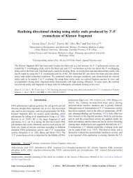
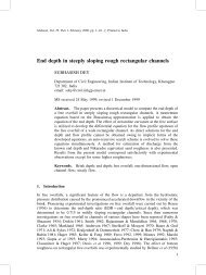
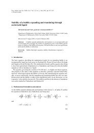
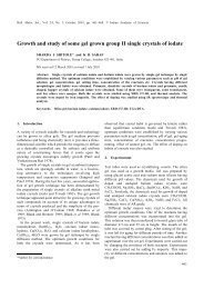
Figure 8. log|s| 2 vs. ω for the states f = 0, 1 and 2 for β = 9, F = 0.05, g = 0,
T = π and i = 0.
decreasing amplitude. The following results are evident from eqs (32b) and (32c) and
figure 8. The quantity s consists of only r 1+ and r 1− . We have ω 00 = 0, ω 10 = 2 and
ω 20 = 3. Consequently, for the states f = 0, 1 and 2 the quantity r 1+ can be neglected
when ω ≈ 0, 2 and 3 respectively because the denominator in r 1− is ≈0. Thus, the firstorder
transition probability for the states f = 0, 1 and 2 becomes maximum at ω = 0, 2
and 3 respectively. For ω ≈ 0 the values of |s| 2 for f = 0, 1 and 2 are ≈ 4F 2 π 2 , 0 and
16F 2 /9 respectively. The first-order transition probability for the state f = 1is≈0. For
the f = 0 state |s| 2 = 0 when ω = 1, 2,...and it becomes maximum when ω = n + 1 2 ,
n = 1, 2,.... When f = 1atω = 4, 6,...the numerators in both r 1+ and r 1− become
zero and thus the quantity |s| 2 is minimum. For f = 2, at odd integer values of ω except
at ω = 3, r 1± = 0 and hence |s| 2 becomes minimum.
Next, we include the high-frequency field and vary its amplitude g and the frequency
. Figure 9 presents the results for a few fixed values of ω with = 5ω. When ω = 1, in
eq. (32b), r 1+ + r 1− = 0 and r 2+ + r 2− = 0for f = 0 and 2 and hence the increase of g
has no effect on |s| 2 .Forthe f = 1 state we find s = (8/3)F − (8/21)g. Asg increases
|s| 2 decreases from (8/3)F, becomes 0 at g = 7F(= 0.35) and then increases with
further increase in g as shown in figure 9a. The first-order transition probability of the
state f = 1 exhibits antiresonance at g = 0.35. Antiresonance can be realizable for other
states also for appropriate choices of ω. For example, in figures 9b and c corresponding
to ω = 1.7 and 2 respectively we can clearly notice antiresonance for f = 0 and 2 states.
In figure 9d where ω = 3.5 the quantity |s| 2 increases monotonically with the control
parameter g for all the three states.
As r 2+ and r 2− (given by eq. (32c)) contain terms which are sinusoidal functions of
, the first-order transition probability can exhibit a sequence of resonance peaks when
is varied for fixed values of other parameters. This is shown in figure 10 for four sets
of values of ω and g. In all the cases is varied from 5ω. In figures 10a–c, |s| 2 = 0
at the starting value of for the f = 0 state. |s| 2 ̸= 0 for wide ranges of values of .
Transition probability of all the states show a sequence of resonance peaks. In figure 10d
|s| 2 of f = 0 state is close to its values of the other two states. However, as increases
|s| 2 of the f = 1 and f = 2 states oscillate but ̸=0. In contrast to this, |s| 2 of the f = 0
state becomes 0 at certain values of .
It is noteworthy to compare the effect of high-frequency external force in the classical
and quantum mechanical Morse oscillators. A classical nonlinear system can exhibit a
138 Pramana – J. Phys., Vol. 81, No. 1, July 2013