Vibrational resonance in the Morse oscillator - Indian Academy of ...

Vibrational resonance in the Morse oscillator
Then
Q 4 = 4 π
1
√(ω 2 r,4 − ω2 ) 2 + d 2 ω 2 . (23)
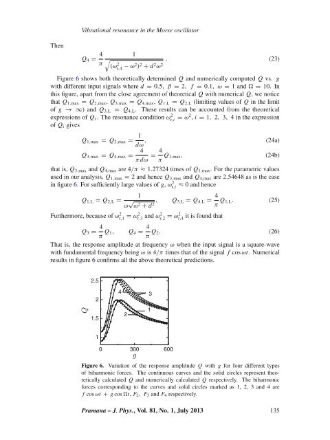
Figure 6 shows both theoretically determined Q and numerically computed Q vs. g
with different input signals where d = 0.5, β= 2, f = 0.1, ω= 1 and = 10. In
this figure, apart from the close agreement of theoretical Q with numerical Q, we notice
that Q 1,max = Q 2,max , Q 3,max = Q 4,max , Q 1,L = Q 2,L (limiting values of Q in the limit
of g → ∞) and Q 3,L = Q 4,L . These results can be accounted from the theoretical
expressions of Q i . The resonance condition ωr,i 2 = ω 2 , i = 1, 2, 3, 4 in the expression
of Q i gives
Q 1,max = Q 2,max = 1
dω ,
(24a)
Q 3,max = Q 4,max = 4
πdω = 4 π Q 1,max,
(24b)
that is, Q 3,max and Q 4,max are 4/π ≈ 1.27324 times of Q 1,max . For the parametric values
used in our analysis, Q 1,max = 2 and hence Q 3,max and Q 4,max are 2.54648 as is the case
in figure 6. For sufficiently large values of g, ωr,i 2 ≈ 0 and hence
1
Q 1,L = Q 2,L =
ω √ ω 2 + d , Q 2 3,L = Q 4,L = 4 π Q 1,L. (25)
Furthermore, because of ωr,1 2 = ω2 r,3 and ω2 r,2 = ω2 r,4
it is found that
Q 3 = 4 π Q 1, Q 4 = 4 π Q 2. (26)
That is, the response amplitude at frequency ω when the input signal is a square-wave
with fundamental frequency being ω is 4/π times that of the signal f cos ωt. Numerical
results in figure 6 confirms all the above theoretical predictions.
2.5
2
1.5
4
2
3
1
1
0
300
600
Figure 6. Variation of the response amplitude Q with g for four different types
of biharmonic forces. The continuous curves and the solid circles represent theoretically
calculated Q and numerically calculated Q respectively. The biharmonic
forces corresponding to the curves and solid circles marked as 1, 2, 3 and 4 are
f cos ωt + g cos t, F 2 , F 3 and F 4 respectively.
Pramana – J. Phys., Vol. 81, No. 1, July 2013 135