The Finite Element Method for the Analysis of Non-Linear and ...
The Finite Element Method for the Analysis of Non-Linear and ...
The Finite Element Method for the Analysis of Non-Linear and ...

You also want an ePaper? Increase the reach of your titles
YUMPU automatically turns print PDFs into web optimized ePapers that Google loves.
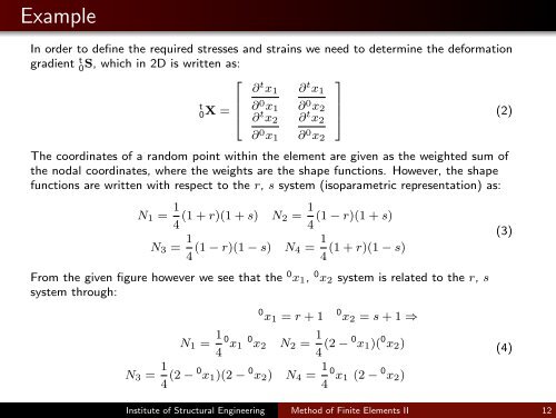
Example<br />
In order to define <strong>the</strong> required stresses <strong>and</strong> strains we need to determine <strong>the</strong> de<strong>for</strong>mation<br />
gradient t 0S, which in 2D is written as:<br />
⎡<br />
∂ t x 1 ∂ t ⎤<br />
x 1<br />
t<br />
0 X = ⎢ ∂ 0 x 1 ∂ 0 x 2<br />
⎣ ∂ t x 2 ∂ t ⎥<br />
x 2 ⎦ (2)<br />
∂ 0 x 1 ∂ 0 x 2<br />
<strong>The</strong> coordinates <strong>of</strong> a r<strong>and</strong>om point within <strong>the</strong> element are given as <strong>the</strong> weighted sum <strong>of</strong><br />
<strong>the</strong> nodal coordinates, where <strong>the</strong> weights are <strong>the</strong> shape functions. However, <strong>the</strong> shape<br />
functions are written with respect to <strong>the</strong> r, s system (isoparametric representation) as:<br />
N 1 = 1 4 (1 + r)(1 + s) N 2 = 1 (1 − r)(1 + s)<br />
4<br />
N 3 = 1 4 (1 − r)(1 − s) N 4 = 1 (3)<br />
4 (1 + r)(1 − s)<br />
From <strong>the</strong> given figure however we see that <strong>the</strong> 0 x 1 , 0 x 2 system is related to <strong>the</strong> r, s<br />
system through:<br />
0 x 1 = r + 1<br />
0 x 2 = s + 1 ⇒<br />
N 1 = 1 4 0 x 1 0 x 2 N 2 = 1 4 (2 − 0 x 1 )( 0 x 2 )<br />
(4)<br />
N 3 = 1 4 (2 − 0 x 1 )(2 − 0 x 2 ) N 4 = 1 4 0 x 1 (2 − 0 x 2 )<br />
Institute <strong>of</strong> Structural Engineering <strong>Method</strong> <strong>of</strong> <strong>Finite</strong> <strong>Element</strong>s II 12